ML Interview Q Series: Geometric Probability: Distribution of Distance to Nearest Rectangle Side

Browse all the Probability Interview Questions here.

You choose at random a point inside a rectangle whose sides have the lengths 2 and 3. Let the random variable X be the distance from the point to the closest side of the rectangle. What is the probability density of X? What are the expected value and the standard deviation of X?

Short Compact solution

The possible values of X range from 0 to 1. For 0 ≤ x ≤ 1, the area of the set of points whose distance to any side exceeds x is (3 - 2x)(2 - 2x). Hence the cumulative distribution function for X is

Differentiating gives the probability density function for 0 < x < 1:

The expected value is

and the second moment is 2/9, leading to variance 2/9 − (7/18)² = 23/324. Therefore the standard deviation is

Comprehensive Explanation

Geometric setup and definition of X

Consider a 2-by-3 rectangle in the plane. If we pick a point uniformly at random inside this rectangle, the random variable X is defined as the distance from that point to the closest side. Because the rectangle is 2 units in one dimension and 3 units in the other, the maximum possible distance to a side occurs if the point is right in the center in the smaller dimension. For this rectangle, the distance to the closest side can never exceed 1, because half of the smaller side is 1.

Derivation of the distribution

A helpful geometric approach is to consider the subset of points inside the rectangle whose distance to any side is greater than some value x. If x is between 0 and 1, these points form a smaller rectangle in the center, having dimensions (3 − 2x) by (2 − 2x). That happens because we must move x inward from each side of the original rectangle, reducing the length of each side by 2x.

The total area of the original rectangle is 6. The area of the smaller rectangle (points with distance > x) is (3 − 2x)(2 − 2x). Hence the probability that X > x is that smaller-area fraction of the total, i.e. ((3 − 2x)(2 − 2x)) / 6. Therefore,

P(X > x) = (3 − 2x)(2 − 2x) / 6,

and the cumulative distribution function is

P(X ≤ x) = 1 − P(X > x) = 1 − [(3 − 2x)(2 − 2x)] / 6.

Expanding (3 − 2x)(2 − 2x) = 6 − 3(2x) − 2(2x) + (2x)(2x) = 6 − 6x − 4x + 4x² = 6 − 10x + 4x². Carefully rewriting, the CDF is:

P(X ≤ x) = [6 − (6 − 10x + 4x²)] / 6 = (10x − 4x²) / 6 = 5/3 x − 2/3 x²,

for 0 ≤ x ≤ 1. Outside that interval, P(X ≤ x) would be 0 if x < 0 and 1 if x > 1.

To find the probability density function, we differentiate:

f(x) = d/dx [5/3 x − 2/3 x²] = 5/3 − 4/3 x.

This pdf applies for 0 < x < 1 and is 0 otherwise.

Checking that f(x) is a valid pdf

We can confirm that integrating f(x) from 0 to 1 gives 1:

∫ from 0 to 1 of (5/3 − 4/3 x) dx = [5/3 x − 2/3 x²]_0^1 = (5/3) − (2/3) = 1.

Expected value of X

We calculate E(X) as:

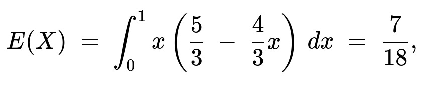
E(X) = ∫ from 0 to 1 of x * f(x) dx = ∫ from 0 to 1 of x (5/3 − 4/3 x) dx.

Compute separately:

∫ from 0 to 1 of (5/3 x) dx = 5/3 * (1/2) = 5/6, ∫ from 0 to 1 of (4/3 x²) dx = 4/3 * (1/3) = 4/9.

Hence E(X) = 5/6 − 4/9 = 15/18 − 8/18 = 7/18.

Variance and standard deviation

To find the variance, we need E(X²). We compute:

E(X²) = ∫ from 0 to 1 of x² (5/3 − 4/3 x) dx.

Compute separately:

∫ from 0 to 1 of (5/3 x²) dx = 5/3 * (1/3) = 5/9, ∫ from 0 to 1 of (4/3 x³) dx = 4/3 * (1/4) = 1/3.

Hence E(X²) = 5/9 − 1/3 = 5/9 − 3/9 = 2/9.

Thus the variance Var(X) = E(X²) − [E(X)]² = (2/9) − (7/18)². Since (7/18)² = 49/324 and 2/9 = 72/324, the difference is 23/324. Taking the square root:

σ(X) = sqrt(23/324) = sqrt(23)/18.

This confirms the standard deviation.

Potential Follow-up Questions and Answers

How does one confirm this density integrates to 1 if one does not trust the algebraic manipulations?

A practical technique is to perform a simple numerical check using a programming language. One can sample many points uniformly in the 2-by-3 rectangle, compute the distance to the closest side, and build an empirical histogram. Compare that histogram with the theoretical pdf = (5/3 − 4/3 x) for x in [0,1]. They should align well for large sample sizes. Alternatively, one can use a symbolic or numerical integration library to integrate f(x) = 5/3 − 4/3 x from x=0 to x=1 and see that it equals 1.

How might we sample X directly from this distribution in a simulation?

An exact approach can use inverse transform sampling. If we let U be uniform(0,1), we can solve P(X ≤ x) = U, i.e. 5/3 x − 2/3 x² = U. That is a quadratic in x: 2/3 x² − 5/3 x + U = 0, or rewriting x² − (5/2) x + (3/2)U = 0. One can solve for x using the quadratic formula and pick the solution consistent with 0 ≤ x ≤ 1. Alternatively, one can simulate a point uniformly in the 2-by-3 rectangle and simply measure its distance to the boundary.

How would these ideas generalize to a rectangle with different side lengths?

If the rectangle had sides of lengths a and b, with a ≤ b, then the maximum distance from a point to a side would be a/2. The random variable X would range from 0 to a/2. All subsequent geometric considerations would be similar, except the smaller rectangle formed by points whose distance exceeds x has side lengths (b − 2x) and (a − 2x). One can replicate the same reasoning to derive a new pdf.

How can we implement a quick code snippet to verify the result numerically?

It is possible to do a simple Monte Carlo test:

import numpy as np

N = 10_000_000
points = np.random.rand(N, 2)
points[:,0] *= 3  # scale x dimension to [0,3]
points[:,1] *= 2  # scale y dimension to [0,2]

dists = np.minimum(np.minimum(points[:,0], 3 - points[:,0]),
                   np.minimum(points[:,1], 2 - points[:,1]))

empirical_mean = np.mean(dists)
empirical_std = np.std(dists, ddof=1)

print("Empirical mean:", empirical_mean)
print("Empirical std:", empirical_std)

Since we know theoretically E(X) = 7/18 and std(X) = sqrt(23)/18, these empirical estimates should converge to approximately 0.3888... and 0.3188... respectively with a sufficiently large sample size.

How does one handle boundary conditions with X=0 or X=1?

The probability that X=0 exactly is 0 in a continuous setting, because picking a point exactly on a boundary is a measure-zero event. Similarly, the chance that X=1 is also 0, because only points precisely at the midline of the 2-by-3 rectangle in the shorter dimension (if the rectangle were 2 by 3) would yield distance 1, and that set also has measure zero in a 2D region. Hence in practical or coding scenarios, we rarely see exact occurrences for these extremes in floating-point arithmetic.

How can we check intuitively that the mean is indeed around 0.3888?

An intuitive check is to realize that the average distance from the boundary cannot be too large since the rectangle’s shorter side is 2. The maximum distance is 1, but most points will not lie near the center line (in the shorter dimension) uniformly. The geometry-based calculation matches well with the integral approach, giving a plausible average distance that is less than half of the rectangle’s half-width.

These details demonstrate both geometric reasoning and confirm consistency with the fundamental principles of continuous probability distributions.

Below are additional follow-up questions

How can we approach the distribution derivation using a direct double integral, and what subtleties might arise?

A direct double integral approach bypasses the geometric area method and instead defines X = distance to the closest side. For each x in [0, 1], we can attempt to integrate over all points whose distance to the boundary is exactly in a small range around x, then sum (integrate) that quantity over x. Formally, one might write:

f(x) = (1 / Area_of_rectangle) * (Area of points whose distance to the boundary lies in [x, x + dx]) / dx,

and let dx → 0. In practice, to perform this integral directly in Cartesian coordinates, one would have to describe the region of points satisfying x ≤ distance_to_closest_side < x + dx. This corresponds to the “shell” formed between two smaller rectangles: one with an offset of x from each side and another with an offset of x + dx from each side.

The subtlety here is in precisely defining that shell and taking care not to double-count points near corners. Each side of the rectangle contributes to the boundary condition for the “closest distance.” Overlapping constraints from adjacent sides can make the region’s shape more complicated if we do not rely on the simpler “shrunken rectangle” approach. One can still do it, but carefully setting up the integrals and ensuring that the boundary shapes do not create extra complexities near corners is nontrivial. This complexity is precisely why a geometric approach (the area of the smaller rectangle) is cleaner in practice.

A pitfall is to forget that the distance to the closest side is not necessarily the distance to the vertical sides or horizontal sides alone. Attempting to integrate incorrectly, for example by summing distance distributions to each side individually, leads to overcounting or ignoring corner regions. The geometry-based approach with (3 - 2x)(2 - 2x) neatly avoids this pitfall.

Could changing the orientation or applying a linear transformation to the rectangle alter the distribution?

If one merely rotates the rectangle in the plane or shifts its origin, the distribution of X remains the same. The reason is that distance to a boundary is preserved under rigid transformations (rotations, translations), and uniform sampling remains uniform under those transformations.

However, if you apply a more general linear transformation that stretches or shears the rectangle, the distribution of X to the boundary can change. Suppose a transformation rescales the rectangle in one dimension but not the other. The side lengths are effectively altered, and so the maximum distance to the nearest side as well as the shape of the “shrunken rectangle” changes. Consequently, the resulting pdf for X would also be different. Indeed, under a uniform sampling in that new coordinate system, the region describing “distance > x” from each boundary would reflect the new side lengths.

An edge case is if the linear transformation skews the rectangle heavily so that it’s no longer axis-aligned. In a purely geometric sense, “distance to a side” is still the perpendicular distance to a line bounding the parallelogram, but if one incorrectly measures “horizontal or vertical distance” after a shear transformation, the distribution is no longer the same as the true perpendicular distance. This highlights the subtle real-world pitfall: always ensure you measure the actual Euclidean distance to the boundary, not just one coordinate difference.

Why does the distribution remain continuous at x = 0 and x = 1, and what could cause discontinuities in other problems?

For a continuous distribution in a 2D area, the probability of exactly being on the boundary (x = 0) or at the maximum possible distance (x = 1 in this rectangle) is zero, so there is no jump in the CDF at these values. The CDF transitions smoothly from P(X ≤ 0) = 0 to P(X ≤ 1) = 1 with no jumps.

Discontinuities in a distance-based distribution to a boundary can arise in different geometries—for instance, if you are dealing with a polygon that has re-entrant corners or non-simply-connected regions (like a rectangle with a hole in the center). If the shape’s boundary changes abruptly or if regions exist where the distance function “jumps,” the distribution might display discontinuities or piecewise behaviors. Another situation might be if the problem defines a discrete mixture of shapes, so that, for example, part of the time you sample points from one shape and part of the time from another. Then you could see a step in the CDF due to the mixture. None of that applies to a simple rectangle, which is why the distribution is continuous for 0 < x < 1.

Could we have accidentally computed the distance to the furthest side instead of the closest side, and how would that change the result?

A common pitfall is mixing up “closest side” vs. “farthest side.” If we picked X to be distance to the farthest side, then the maximum possible distance could be up to 3 if the rectangle is 2 by 3, but we would need to reason carefully which dimension is bigger. In fact, for a 2-by-3 rectangle, the farthest side from a given point might be one of the vertical boundaries or one of the horizontal boundaries, depending on where you stand.

That distribution would be completely different because you would effectively look at 2 - distance from one dimension or 3 - distance from the other dimension. The geometry-based approach that simply “shrinks” the rectangle by 2x on each dimension no longer applies in a straightforward manner for “farthest side.” Instead, you would consider an “offset boundary” outward rather than inward, which is not possible for a rectangle in the plane. You would end up with a different bounding geometry for valid points. Ultimately, for the given problem about “closest side,” you must be certain you are shrinking the rectangle rather than expanding it. Confusing these two leads to a drastically different distribution.

How might random sampling errors or uniformity concerns alter real-world estimates for X?

If, in a real application, points inside the rectangle are sampled in a manner that is not strictly uniform (e.g., the random generator is biased or subregions are more likely to be chosen), the observed empirical distribution for X will deviate from the theoretical pdf. In machine learning applications, for instance, if the rectangle represents some bounding box of data samples, and the samples are physically collected in a non-uniform way, X might appear to have a distribution narrower or wider than the theoretical one.

A subtlety is that in computational settings, pseudo-random number generators can exhibit correlations if not used carefully, especially for very large sample sizes or in parallel computing contexts. This can skew the observed distribution of distances. Additionally, floating-point precision issues might become relevant if the rectangle is extremely large or extremely small compared to the machine’s floating precision. Hence, verifying uniform sampling in code and ensuring that the scale of the rectangle remains within a stable numeric range is essential to prevent anomalies or artifacts in the estimated distribution.

What if we had chosen a narrower rectangle, say 1 by 3, where the maximum distance from a side is 0.5?

If the rectangle is 1 by 3, the smaller dimension is now 1, so the maximum possible value for X is 0.5. The general formula for the distribution can still be derived using the approach of “shrinking the rectangle by 2x.” Specifically, for a rectangle of lengths a and b with a < b, the subset of points at least x away from any side is (b - 2x)(a - 2x), for x in [0, a/2]. Dividing by the total area ab gives the probability that the distance is at least x. One then obtains the distribution by 1 - that expression. As soon as a is changed from 2 to 1, the upper bound for X changes from 1 to 0.5, altering the integral limits and the final function.

A pitfall would be to forget to adjust for a new maximum distance if the smaller side is changed. People sometimes keep the same formula for x in [0,1], but if the rectangle is only 1 unit in one dimension, that formula becomes invalid for x > 0.5. Always ensure that the “range of X” matches half the smaller side.

How does the existence of corners (as opposed to a circle or oval boundary) simplify this problem?

Corners in a rectangle mean the boundary is composed of four line segments. If we wanted the distance to the closest side, we just need to consider orthogonal (perpendicular) distances to each of these line segments, which is straightforward—particularly because the rectangle’s edges do not curve. With a circular or elliptical boundary, the geometry of “closest side” is replaced by “closest point on a curve,” which typically complicates direct area-based arguments. Instead, we might require polar coordinates or advanced integration to find the region of points at least x away from that boundary.

An important real-world subtlety is that corners do not add “extra distance constraints” for “closest side” beyond the lines themselves. The corner might represent the closest point on the boundary, but from an area perspective, corners do not create a separate zone of constant distance (they are measure-zero sets in continuous space). The rectangle’s side-based offset concept remains clean. In a circle or an irregular polygon, we cannot simply shift each side by x to form a smaller shape: we must shift the entire boundary, including curved arcs, which is more involved.

What if the problem asked for the joint distribution of distances to both the horizontal side and the vertical side?

This changes the question significantly. Define Y = distance to the nearest horizontal side and Z = distance to the nearest vertical side. Now X = min(Y, Z) is just one aspect. If we wanted their joint distribution (Y, Z), then the uniform sampling inside a 2-by-3 rectangle implies Y in [0,1] (since the half-height is 1) and Z in [0,1.5] (since the half-width is 1.5). One could write:

Y = distance to horizontal side = min(y, 2 - y), Z = distance to vertical side = min(x, 3 - x),

assuming the rectangle corners are at (0,0), (3,0), (3,2), (0,2). Then (Y, Z) is not uniformly distributed in its bounding box [0,1] × [0,1.5], because the mapping from (x,y) → (Y,Z) is not linear. Determining the joint pdf would involve a Jacobian of the transformation from (x,y) to (Y,Z) or carefully dissecting the rectangle into regions where Y = y vs. Y = 2 - y, etc.

A pitfall is to assume Y and Z are independent. They are not, because their definitions both depend on the particular location of the point in the rectangle. For example, if a point is near the left edge (making Z small), that does not automatically force Y to be small or large, but certain corners or side constraints can produce correlations. So if an interviewer asked about the joint distribution, the main challenge is to handle the piecewise nature of how Y and Z are determined from the raw coordinates and then track the area mapping carefully.

What are typical mistakes students make in a timed exam or interview when tackling this problem?

One common mistake is mixing up the geometric “shrunken rectangle” area with something else, like subtracting incorrectly or forgetting to scale by the original area. Another error is forgetting that the rectangle’s smaller side is 2, so the maximum distance to a side is 1, not 2 or 3. Also, some might incorrectly assume the distribution is uniform in [0,1], forgetting the geometric constraints.

A more subtle error is failing to differentiate the CDF properly to obtain the PDF or forgetting to multiply by the negative sign if one tries to do it as f(x) = - d/dx of (area ratio) for the region distance > x. It’s easy to get sign errors.

Finally, a conceptual pitfall is ignoring corner cases such as x=0 or x=1, or misinterpreting them as having some finite probability. Since this is a continuous distribution, the probability that X exactly hits those endpoints is zero. In a real interview, emphasizing these clarifications shows the candidate understands the measure-theoretic and geometric subtleties of continuous random variables.