
ML Interview Q Series: Geometric Queue & Conditional Expectation: Finding Your Message's Expected Transmission Position.

Browse all the Probability Interview Questions here.
In a buffer there is a geometrically distributed number of messages waiting to be transmitted over a communication channel, where the parameter p of the geometric distribution is known. Your message is one of these waiting messages. The messages are transmitted one by one in random order. Let the random variable X be the number of messages that are transmitted before your message. What are the expected value and the standard deviation of X?
Short Compact solution
From the given setup, if Y denotes the total (geometrically distributed) number of messages in the buffer, then conditional on Y = y, your message’s position among those y messages is uniformly distributed over the y possible positions. Hence the conditional expectation of X, the number of messages transmitted before yours, is (y - 1)/2. Averaging this over the distribution of Y leads to:

A more detailed analysis (using the conditional variance of a discrete uniform distribution and then taking the expectation over Y) shows that the standard deviation of X is:

Comprehensive Explanation
Understanding the setup There are Y messages in the buffer, where Y follows a geometric distribution with parameter p. By convention, this means that the probability Y = y is p(1-p)^(y-1) for y >= 1. Among these y messages, yours is equally likely to occupy any of the y “positions” in the random transmission order.
Defining X We let X be the number of messages transmitted before your message. If Y = y, then there are y total messages, and your message could appear in any of the positions 1 through y with equal probability 1/y. Hence X is uniformly distributed between 0 and y - 1 (because if you are in position k, then k - 1 messages are ahead of you, but letting X = k - 1 means X ranges from 0 through y - 1).
Conditional expectation When Y = y, X has a discrete uniform distribution on 0,...,y - 1. The mean of a discrete uniform(0,...,m - 1) is (m - 1)/2, so
E(X | Y = y) = (y - 1)/2.
Taking the overall expectation We then take the expectation of E(X | Y = y) over the distribution of Y. The random variable Y has mean 1/p, so
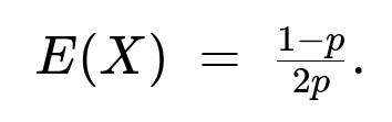
E(X) = E( (Y - 1)/2 ) = (1/2) ( E(Y) - 1 ) = (1/2) ( (1/p) - 1 ) = (1 - p)/(2p).
Hence,
Variance and standard deviation To find the standard deviation, we use:
Var(X) = E( Var(X | Y) ) + Var( E(X | Y) ).
The conditional variance of X given Y = y, for X ~ discrete uniform(0,...,y-1), is (y^2 - 1)/12.
The conditional mean is (y - 1)/2, so its square is (y - 1)^2 / 4.
Putting these together to get E(X^2) = E( Var(X | Y) ) + E( [E(X | Y)]^2 ), then subtracting [E(X)]^2 yields Var(X). The resulting algebra leads to:
Var(X) = ( (1-p)(p + 5 ) ) / (12 p^2 ).
Taking the square root gives the standard deviation:

Potential Follow-up questions
How does the fact that Y is geometric influence the distribution of X compared to if Y were fixed? If Y were a fixed number (say Y = n deterministically), then X would be uniformly distributed on 0,...,n - 1. Its expected value would simply be (n - 1)/2, and its variance would be (n^2 - 1)/12. However, because Y is itself random (with a geometric distribution), we take a further expectation over Y, which modifies the mean and variance. This “two-layer” approach is an instance of the law of total expectation and the law of total variance.
Why is E(X) = (1-p)/(2p)? Intuitive interpretation? Since Y has an average of 1/p messages, on average there are 1/p messages in the buffer, so on average there are 1/p - 1 other messages besides yours. If your message’s position is random among them, you would expect roughly half of those 1/p - 1 messages to come before you, leading to the factor of 1/2 in the result.
Could you derive E(X) without explicitly summing series? Yes. One approach is to use the law of total expectation directly: E(X) = E( E(X|Y) ). Given Y = y, X ~ discrete uniform(0,...,y-1), so E(X|Y=y) = (y - 1)/2. Then E(X) = (1/2) E(Y - 1) = (1/2)( E(Y) - 1 ), and since E(Y) = 1/p for a geometric distribution with parameter p, the final result is (1/2)(1/p - 1).
Why is the standard deviation not just half of the standard deviation of Y? Your message is not waiting among all Y messages in a linear fashion—rather, its position is a uniform random draw among Y positions, and that “uniform position” adds its own variance structure on top of the fact that Y itself is random. This combination leads to a formula that incorporates the variance of Y (which is (1-p)/p^2) and the variance of a discrete uniform distribution, requiring the use of the law of total variance to get the final result.
How might you simulate this in Python to verify the result? You could perform a Monte Carlo simulation:
Generate Y from a geometric distribution with parameter p.
Simulate a random position for your message among those Y messages, effectively picking X uniformly on 0,...,Y-1.
Collect a large number of samples of X and then compute the empirical mean and standard deviation to compare with the derived formulas.
A simple implementation sketch:
import numpy as np

def geometric_sample(p):
    # Generate one sample from a geometric(p) with support {1, 2, 3, ...}
    # Using NumPy's built-in might differ slightly in parameterization, so we do this custom:
    count = 0
    while True:
        count += 1
        if np.random.rand() < p:
            return count

def simulate_X(num_samples, p):
    samples = []
    for _ in range(num_samples):
        y = geometric_sample(p)
        x = np.random.randint(0, y)  # Uniform on [0, y-1]
        samples.append(x)
    return np.mean(samples), np.std(samples)

p = 0.3
mean_est, std_est = simulate_X(10_000_00, p)
print("Estimated E(X):", mean_est)
print("Estimated Std(X):", std_est)

# Compare with the formulas:
E_X = (1 - p) / (2 * p)
Std_X = np.sqrt((1 - p) * (p + 5) / (12 * p**2))
print("Analytical E(X):", E_X)
print("Analytical Std(X):", Std_X)
Such a simulation would confirm the correctness of the derived expressions for E(X) and std(X) as the number of trials grows.
Below are additional follow-up questions
What happens if the parameter p of the geometric distribution is extremely small or extremely large?
If p is extremely small, the geometric random variable Y (the total number of messages in the buffer) tends to have a very large expected value 1/p. Intuitively, with a small p, the probability of having a “success” in the geometric sense is very low, so on average you see many messages in the buffer. Consequently, your expected X becomes (1-p)/(2p) which can be quite large when p is small. This aligns with the idea that if the buffer is huge, a random transmission order is more likely to place your message somewhere among many others waiting, so the number of messages before yours (X) can be large.
Conversely, if p is very large (close to 1), Y is most likely equal to 1 (or very small), meaning very few messages are in the buffer on average. Thus X is likely to be 0 much of the time, because with high probability your message is the only one or one of very few. In that regime, (1-p)/(2p) becomes small. The standard deviation also shrinks when p is high, because the distribution of X is then concentrated at lower values.
Pitfalls and edge cases:
Floating-point issues in code: When p is extremely small or extremely large, we might get numerical overflow or underflow when computing p(1-p)^(y-1). We must handle that carefully in simulation.
Misinterpretation of Y’s scale: If engineers expect Y to be small but p is actually small, the system capacity might be underestimated in real-world scenarios.
Could the memoryless property of the geometric distribution affect how we treat conditional expectations?
The geometric distribution is memoryless in the sense that P(Y > k + r | Y > k) = (1-p)^r. This property sometimes simplifies certain derivations because it lets us condition on events like “Y > k” without complicating the tail distribution. In the specific approach to computing E(X) or Var(X), we used the law of total expectation and the discrete-uniform property of your message’s position conditional on Y, rather than directly using memorylessness. However, if we tried to compute some probabilities about the ordering of messages after partial transmissions, the memoryless property would simplify the analysis of “how many messages remain” after k transmissions.
Pitfalls and edge cases:
In certain alternative derivations, ignoring the memoryless property can lead to more complex summations. Memorylessness often gives shortcuts but is not strictly mandatory for the approach used here.
If we replaced the geometric distribution by another distribution (e.g., Poisson or negative binomial) that is not memoryless, the same method of conditioning on Y’s realized value still works, but we cannot use memorylessness to simplify the tail distribution.
What if we impose a different transmission policy instead of random order?
In the given question, the order is chosen at random among the Y messages. Suppose we use a deterministic policy, like first-in-first-out (FIFO). Then if your message arrives last, that would force you to wait for all previously arrived messages. In that case, X’s distribution would be related to arrival order instead of a random permutation among Y.
Pitfalls and edge cases:
If the scheduling policy is priority-based or FIFO-based, X might be determined by arrival times, not a uniform random ordering. The distribution of X would then depend on the arrival process, so the uniform distribution assumption of your position among Y messages would no longer hold.
Using a random order might seem artificial, but in some real systems (like random backoff protocols in networking), the effective order can indeed appear randomized.
How do you verify correctness if you only have partial information about Y or p in a real system?
In practice, you may not know p precisely or may only see the realized values of Y occasionally. To check if your theoretical formulas match reality, you could:
Estimate p by monitoring how many messages are typically in the buffer (the sample mean of Y) and invert to find an empirical p_est ~ 1 / (mean of Y).
Collect statistics on X across many transmissions (e.g., how many messages were observed to be transmitted before yours in each scenario). Compare the empirical mean and standard deviation of X with the theoretical (1-p)/(2p) and sqrt(((1-p)(p+5)) / (12p^2)). If they align closely, that supports correctness.
Pitfalls and edge cases:
Noise in measurement: If the system is time-varying or p changes with load, a single estimate of p might not be valid across different time intervals.
Non-geometric arrivals: In real networks, arrival processes might follow bursts, or messages might have correlated arrival times, invalidating the geometric assumption.
Could we encounter boundary cases like Y = 0 or negative Y in practice?
By definition of the geometric distribution (in the form used here), Y takes values in {1, 2, 3,...}. There is no Y = 0. If we wanted a version of the geometric distribution that allows Y = 0 with probability p and Y = k with probability (1-p)^k p for k >= 0, we would have a shifted version of the distribution. In that case, the algebra would change slightly: E(Y) would be (1-p)/p, and so on. But the logic of uniform random ordering among Y messages would remain, just that Y could be zero with some probability, meaning X = 0 automatically.
Pitfalls and edge cases:
Some references define the geometric distribution differently (support {0,1,2,...}). The question’s derivation must be consistent with the definition that Y >= 1.
Implementation detail: If a system can truly have zero messages, one must carefully handle the case Y = 0 (it would mean your message might be the only one that has just arrived).
What if your message is not guaranteed to be among the Y messages?
One assumption in the problem is that “Your message is one of these waiting messages.” In a real scenario, it might arrive at random times. If there’s only a probability of your message being in the queue at a certain sampling instant, or if your message arrives after some have been transmitted, the distribution of X could differ significantly.
Pitfalls and edge cases:
If your message arrives while transmissions are in progress, the set of possible positions for your message is influenced by arrival time, not a uniform distribution among Y.
If your message can fail to show up entirely, we would need to condition on the event your message is indeed present in the buffer, altering the distribution again.
Could the random ordering be correlated with the message’s arrival times or sizes?
In theory, random order is taken as an independent random permutation of the Y messages in the queue. But in many real systems, the order might depend on arrival timestamps, message priorities, or message sizes. For example, a system might schedule short messages first (Shortest Job First) or large messages first in a specialized system. If correlation exists between the message arrival time and its position in the transmission order, the discrete uniform assumption for X given Y is invalid.
Pitfalls and edge cases:
Failing to account for correlation can lead to inaccurate estimates of X or its variance if the system has a biased scheduling discipline.
Some scheduling algorithms approximate random or uniform selection, but real data might reveal slight bias.
If the number of messages Y is drawn from a mixture distribution rather than a single geometric distribution, how would that affect X?
In a mixture, you might have Y ~ w * Geom(p1) + (1-w) * Geom(p2). Then E(X | Y=y) is still (y - 1)/2 if your message is guaranteed to be among y messages with a random permutation. But to get E(X), you must compute an expectation across that mixture distribution for Y. The same law of total expectation approach applies, but the final expression for E(X) and Var(X) becomes a weighted combination of the partial expectations and variances for each component in the mixture.
Pitfalls and edge cases:
Mixture models can increase complexity; the distribution for Y might not have a straightforward closed form, so summations or integrals might be more complicated.
If p is not constant in time, applying a single formula might be misleading. You would need to incorporate the time-varying or mixture nature of arrivals.