
ML Interview Q Series: Geometric Variables: Uniform Conditional Distribution Given Their Sum

Browse all the Probability Interview Questions here.
Let (X_1) and (X_2) be independent random variables each having a geometric distribution with parameter (p). What is the conditional probability mass function of (X_1) given that (X_1 + X_2 = r)?
Short Compact solution
By the convolution formula for two independent geometric random variables, we have

Then,
(P(X_1 = j,, X_1 + X_2 = r)) equals (p(1-p)^{j-1},p(1-p)^{r-j-1} = p^2,\bigl(1-p\bigr)^{r-2}).
Dividing by (P(X_1 + X_2 = r)) yields:

Hence, the conditional distribution of (X_1) given (X_1 + X_2 = r) is uniform on the set ({,1,,2,\dots,,r-1}).
Comprehensive Explanation
Setup and notation
We have two independent random variables (X_1) and (X_2). Each follows a geometric distribution with parameter (p). This means:
(X_1, X_2 \in {1,2,3,\dots}).
For each (i \in {1,2}), (P(X_i = k) = p,(1-p)^{,k-1}) for (k = 1,2,3,\dots).
We want to find the conditional probability (P(X_1 = j \mid X_1 + X_2 = r)).
Convolution and sum distribution
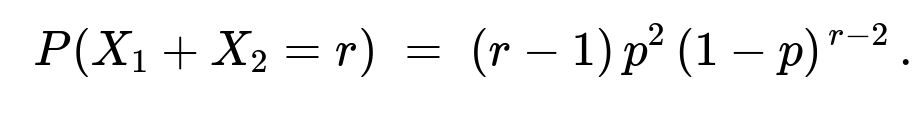
First, we compute (P(X_1 + X_2 = r)). Because (X_1) and (X_2) are independent and geometric, their sum follows a Negative Binomial distribution with parameters (\alpha=2) and (p). However, it is straightforward to do the convolution explicitly:
We consider all pairs ((k,,r-k)) with (k = 1,2,\dots, r-1).
The joint pmf (P(X_1 = k,; X_2 = r-k)) is (p,(1-p)^{,k-1};\cdot;p,(1-p)^{(r-k)-1}).
Summing over (k) from (1) to (r-1) gives:
Each term in the sum is (p^2,(1-p)^{,r-2}).
There are ((r-1)) such terms.
Thus,
Numerator: joint event (X_1 = j, , X_1 + X_2 = r)
When (X_1 = j) and (X_1 + X_2 = r), it must be that (X_2 = r-j). Thus,
(P(X_1 = j,; X_2 = r-j) = p,(1-p)^{,j-1},\times,p,(1-p)^{(r-j)-1} = p^2,(1-p)^{,r-2}).
Putting it all together
By definition of conditional probability:

Plugging in the values:
Numerator: (p^2,(1-p)^{,r-2}).
Denominator: ((r-1),p^2,(1-p)^{,r-2}).
Hence,

This means (X_1) is uniformly distributed over the integers (1,2,\dots,r-1) when we condition on (X_1 + X_2 = r).
Why uniform?
An intuitive reason for the uniformity is related to the memoryless property of the geometric distribution. When you know the sum (X_1+X_2 = r), the “split” between (X_1) and (X_2) becomes equally likely among all valid partitions (as long as both are at least 1). This uniform property is a special case of a broader result that, for sums of i.i.d. memoryless random variables, the conditional distribution of one given their sum is uniform on all feasible values.
Follow-up question 1
Could this result change if we used a different definition for the geometric distribution, for example one that starts at 0 instead of 1?
When some texts define a geometric random variable as the number of failures before the first success, the support becomes ({0,1,2,\dots}). In that case, to compute (P(X_1 + X_2 = r)) or the conditional distribution, you would sum over ((k,,r-k)) where (k) ranges from 0 to (r). You would still end up with a uniform distribution but shifted to ({0,1,\dots,r}) except you have to account for the actual range. Specifically, if both variables are defined on ({0,1,2,\dots}), then ({(k, r-k),|,k=0,\dots,r}). The algebra follows similarly, and you get:
(P(X_1 + X_2 = r) = (r+1),p^2,(1-p)^{,r}).
Then (P(X_1 = j \mid X_1 + X_2 = r) = 1/(r+1)).
Thus the uniform property remains. The only difference is the shift in indexing.
Follow-up question 2
What if we had more than two geometric random variables, say (X_1, X_2, \dots, X_n)? Is a similar statement true for the conditional distribution of one of them, given their sum?
Yes, there is a generalization. If (X_1, X_2, \dots, X_n) are i.i.d. geometric( (p) ) random variables and you condition on (X_1 + X_2 + \dots + X_n = r), the joint distribution of ((X_1,\dots,X_n)) among all integer partitions of (r) with each (X_i \ge 1) is symmetric. Each valid partition ((x_1,\dots,x_n)) with (x_1 + \dots + x_n = r) has the same probability. Then any marginal distribution, such as (X_1) conditional on the sum, becomes the distribution that is uniform over all feasible values (1,2,\dots,r-(n-1)). This is a special case of the “multinomial” perspective for i.i.d. geometric random variables.
Follow-up question 3
If a hiring manager asked you to simulate or verify this in Python, how would you do it?
You can run a simple Monte Carlo simulation:
import numpy as np

p = 0.3
num_samples = 10_000_000
X1 = np.random.geometric(p, size=num_samples)
X2 = np.random.geometric(p, size=num_samples)

r = 5  # Condition on sum == 5
mask = (X1 + X2 == r)
X1_given_sum = X1[mask]

# Estimate empirical frequencies
counts = np.bincount(X1_given_sum)
# We only need the range 1..(r-1), but let's see the distribution:
for j in range(1, r):
    print(f"Value {j}, empirical prob = {counts[j]/counts[1:r].sum():.4f}")
If you run this code, you should see approximately uniform probabilities for 1, 2, ..., (r-1). The uniform distribution emerges clearly for large num_samples.
Follow-up question 4
Why does the memoryless property play such a critical role in achieving uniformity?
The memoryless property for a geometric random variable states that for any (k, m),
(P(X > k + m \mid X > k) = P(X > m)).
When you know that (X_1 + X_2 = r), effectively you are determining how the random total (r) is shared between the two variables. For memoryless random variables (like geometric), the chance of being “the first (j) out of the total (r) events” is the same for each (j) in ({1,2,\dots,r-1}) (assuming they start at 1). Intuitively, from a counting perspective, each way of splitting the sum into two positive integers is equally likely once we fix the sum.
Thus, memorylessness is the core property that leads to the simple discrete-uniform distribution under the given sum condition.
Below are additional follow-up questions
Could the uniform result fail when p is very close to 0 or very close to 1?
When p approaches 1, the probability that X_1 = 1 becomes almost certain, and similarly for X_2. In that extreme limit, the sum X_1 + X_2 is almost always equal to 2. Conditioned on X_1 + X_2 = r > 2, it becomes nearly impossible for such an event to occur, so the conditional pmf has negligible probability in practical terms (the event rarely happens). Conversely, when p approaches 0, we tend to see extremely large values for each X_i. Technically, the formula still holds (the sum distribution is still valid, and the conditional distribution remains uniform over feasible values). However, numerical underflow can arise in finite-precision machines when computing (1-p)^(r-1) for very large r, especially if r is large and 1-p is close to 1. In real-world scenarios where r is high and p is very small, one must implement stable numeric routines (e.g. working in log-space) to avoid floating-point issues. Mathematically, the result that the conditional distribution is uniform does not fail, but practical computation might require care.
What if X_1 and X_2 are geometric but with different success parameters?
Suppose X_1 ~ Geom(p1) and X_2 ~ Geom(p2) with p1 != p2. The sum X_1 + X_2 is no longer governed by a simple negative binomial formula in the same way, because the pmfs differ. Even though the random variables are independent, the uniform result for P(X_1 = j | X_1 + X_2 = r) no longer generally holds. The uniformity heavily relies on each component having the same “memoryless” structure with the same parameter. If p1 != p2, you can still do a convolution, but the expression for the conditional probability is not constant in j. A subtle pitfall is to assume memorylessness alone (without identical parameters) suffices for uniformity. In reality, both independence and identical parameters are crucial.
How does dependence or correlation between X_1 and X_2 affect the conclusion?
The derivation of the uniform conditional distribution uses the assumption that X_1 and X_2 are independent. If they are correlated, even if each is marginally geometric with the same parameter, the conditional pmf given X_1 + X_2 = r is not guaranteed to be uniform. For instance, if there is a strong positive correlation (whenever X_1 is large, X_2 tends to be large too), then given a certain sum r, the distribution of X_1 alone will be skewed according to how the dependence is structured. One might guess that X_1 and X_2 “share” the sum differently from one iteration to the next. A real-world pitfall occurs if someone incorrectly assumes independence in applying the uniform result to correlated random variables, leading to biased or incorrect conclusions.
Can this discrete case be connected to continuous analogs, such as exponential distributions?
Yes, there is a parallel result in the continuous domain. If Y_1 and Y_2 are independent exponential random variables with the same rate parameter λ (exponential is the continuous analogue to the geometric distribution’s memorylessness), then conditioning on Y_1 + Y_2 = s makes (Y_1, Y_2) uniformly distributed along the line y1 + y2 = s in the positive quadrant. In other words, Y_1 / (Y_1 + Y_2) is uniformly distributed on (0, 1). That phenomenon is a direct outcome of the memoryless property of the exponential. The discrete and continuous forms mirror each other. In practice, a pitfall is to conflate the discrete and continuous memoryless results and apply one in the context of the other incorrectly. One must pay attention to whether the data or theoretical context is geometric or exponential to apply the correct formula.
Are there any real-world applications where this conditional uniform distribution plays a practical role?
One domain is queueing theory. Suppose the number of arrivals in a certain time period is modeled by geometric distributions under discrete-time processes. If you know that exactly r customers arrived in two consecutive intervals, the uniform result tells you the distribution of how many arrived in the first interval versus the second. Another domain could be reliability testing where discrete geometric variables might capture the count of trials until failure or success. Given a total number of successes in two separate but similarly parameterized processes, the uniform conditional distribution clarifies how the successes might have been split. A subtlety, however, is that many real-world data-generating processes are only approximately geometric and might have over-dispersion or other complexities. If the data depart from the geometric assumption, the uniform property no longer holds. One pitfall is automatically assuming perfect geometric behavior without conducting model checks.
How might we adapt inference if p is unknown and we only observe X_1 + X_2?
If you only see aggregated data of the form X_1 + X_2 = r for each trial, without separate observations of X_1 and X_2, you lose the ability to distinguish how many were contributed by each variable. As a result, estimating p from only the sum distributions can be more challenging and generally requires methods such as maximum likelihood under the negative binomial structure (with 2 successes) or Bayesian estimation with suitable priors. A subtle pitfall is to assume you can just treat r as “one observation” of a geometric distribution. In reality, you have the sum of two geometrics, so the distribution is negative binomial with parameters (2, p). You must handle the different pmf carefully when deriving an estimator for p.