
ML Interview Q Series: Gradient Checking: Verifying Backpropagation Correctness via Numerical Gradient Approximation.
📚 Browse the full ML Interview series here.
Gradient Checking: When implementing backpropagation from scratch, why is it important to perform gradient checking? *Explain how gradient checking works (comparing analytical gradients to numerical approximations) and how it helps verify the correctness of your implementation.*
Understanding how gradients flow through a neural network is critical for ensuring that a model learns correctly. When you implement backpropagation manually, especially for a more complex model, you can encounter subtle mistakes in matrix multiplications, indexing, or partial derivative calculations. Gradient checking is a procedure that helps verify whether the computed analytical gradients (obtained via backpropagation) are correct by comparing them to numerical estimates of those same gradients.
Below is a deep exploration of why gradient checking is important and how it is done, followed by multiple possible follow-up questions (each in its own heading), with detailed answers to address all nuances and potential pitfalls.
Gradient checking is especially relevant in scenarios such as:
Implementing novel or custom neural network layers where no well-tested library code exists.
Debugging unexpected training behavior (e.g., cost exploding or barely changing).
Ensuring correctness before optimizing the network at scale.
Why Gradient Checking Matters
Gradient-based learning requires correct backpropagation of partial derivatives for each parameter. If the gradient is wrong, your optimization steps will not move you correctly through the parameter space. As a result, your training could fail to converge or converge to suboptimal values. Subtle bugs in backpropagation logic often go unnoticed because the training loop might not outright crash, but the model fails to learn effectively. Gradient checking addresses this by verifying that the analytic gradients match numerical approximations to a reasonable tolerance.
Core Concept Behind Gradient Checking
The main idea is to approximate the gradient of the loss function with respect to a parameter by slightly perturbing that parameter and observing how the loss changes. This involves finite differences. The simplest variant is the central difference formula:
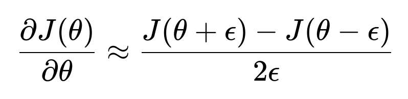
where ( J(\theta) ) is the cost (or loss) function, and ( \epsilon ) is a small number, like ( 10^{-4} ) or ( 10^{-5} ). This approximation is compared to the analytical gradient you computed via backpropagation. If these two gradients match closely (within a small tolerance), it is a good indication that your backpropagation is correct.
Detailed Steps in Performing Gradient Checking
You typically proceed as follows:
Choose a set of parameters to check. Often, you do not need to check every parameter—just a small selection from each layer can be sufficient.
For each chosen parameter:
Save the original parameter value.
Perturb it by ( +\epsilon ) and compute the forward pass to get ( J(\theta + \epsilon) ).
Perturb it by ( -\epsilon ) and compute the forward pass to get ( J(\theta - \epsilon) ).
Compute the numerical gradient using the central difference formula above.
Compare this numerical gradient to the analytical gradient obtained from backpropagation.
Evaluate the difference using a norm metric, for example:
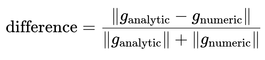
If the difference is on the order of ( 10^{-7} ) or lower (sometimes up to ( 10^{-3} ) or ( 10^{-4} ), depending on the complexity of the model and floating-point precision), your implementation is likely correct.
Code Example in Python (Illustrative)
Below is a simplified snippet that shows the numerical approximation for a single parameter index. Suppose you have a function forward_and_loss(params) that returns the loss:
import numpy as np

def numerical_gradient(params, param_index, epsilon, forward_and_loss):
    """
    params: a numpy array of parameters
    param_index: index of the parameter to perturb
    epsilon: small perturbation
    forward_and_loss: function that takes 'params' and returns a scalar loss
    """
    # Store original value
    original_value = params[param_index]

    # Compute J(theta + epsilon)
    params[param_index] = original_value + epsilon
    loss_plus = forward_and_loss(params)

    # Compute J(theta - epsilon)
    params[param_index] = original_value - epsilon
    loss_minus = forward_and_loss(params)

    # Restore original value
    params[param_index] = original_value

    # Central difference approximation
    grad_approx = (loss_plus - loss_minus) / (2.0 * epsilon)
    return grad_approx
You would compare grad_approx to your analytically computed gradient for param_index.
Potential Pitfalls and Considerations
Choosing Epsilon: If ( \epsilon ) is too large, the finite difference approximation becomes imprecise because higher-order terms are not negligible. If ( \epsilon ) is too small, floating-point rounding can dominate. Typical values are around ( 10^{-4} ) to ( 10^{-6} ).
Regularization: Make sure to incorporate regularization (e.g., penalty) in both the loss function and the backpropagation. Overlooking it in one place causes discrepancies.
Batch vs. Single Example: Sometimes it is easier to do gradient checking on a single example or a small batch to simplify computations and debug. But remember that your final training might use a different approach for batch processing.
High-Dimensionality: Directly checking every single parameter in a large network is computationally expensive. Common practice is to check a small random subset from each layer.
Excluding Gradient Checking from Production: Gradient checking is a debugging and validation technique, not part of the actual training loop. Only do it occasionally, because it is expensive to do for every iteration.
How It Helps Verify Correctness
By comparing the backprop-derived gradient to a numerical approximation, you minimize the chances of systematic errors in your derivation or coding logic. This cross-verification makes it much easier to isolate whether a sudden training issue is due to incorrectly coded backprop or something else (like data preprocessing). If your gradient check passes to a high level of precision, you can proceed with confidence that the backprop implementation is correct.
How Could You Decide on an Appropriate Epsilon Value?
A valid follow-up might ask how to pick ( \epsilon ). The essence is that you want it small enough so that your finite difference formula is accurate, but not so small that floating-point errors overshadow the difference in your function evaluations. A typical range is ( 10^{-4} ) to ( 10^{-7} ). Trying different orders of magnitude and observing the stability of the gradient estimates is a good practice. You can also use the central difference approach to reduce error versus a simple forward difference scheme.
When you pick your ( \epsilon ), you are looking for a “sweet spot”:
If ( \epsilon ) is too large, you are approximating the slope over a big interval, losing the fidelity of the local derivative.
If ( \epsilon ) is too small, floating-point rounding errors in computing ( J(\theta + \epsilon) ) and ( J(\theta - \epsilon) ) can overwhelm the difference.
How Do You Manage the Computation Overhead of Gradient Checking?
It can be expensive to do a forward pass multiple times for every single parameter. Strategies to mitigate this include:
Checking a small random subset of parameters (e.g., 10-20 parameters in each layer) rather than every one.
Checking only once before major training runs, or when debugging suspicious gradient behavior.
Sometimes using automatic differentiation libraries (like PyTorch or TensorFlow) to ensure correctness in gradient calculations, which reduces the need for manual gradient checks, though in research or novel layer scenarios, manual checks can still be invaluable.
What Are Some Typical Tolerances for the Gradient Check?
One common approach is to look at a relative difference measure:
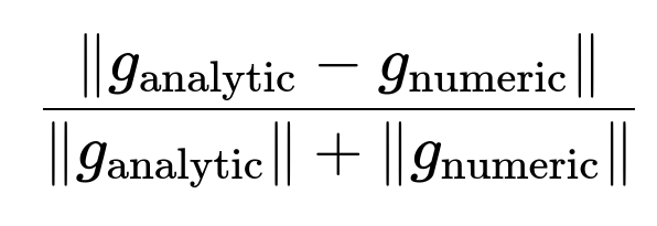
If this value is on the order of ( 10^{-7} ) or lower, your gradient implementation is very likely correct. Sometimes up to ( 10^{-3} ) or ( 10^{-4} ) may be acceptable in practice—especially in large-scale networks—because floating-point errors and the complexity of computations can make very tight tolerances hard to achieve.
Could You Accidentally Pass Gradient Checking While Still Having a Bug?
Yes, there are rare cases. For instance, if you have symmetrical errors that mask each other across different parameters, your local checks might not catch them. Also, failing to incorporate certain regularization components in both numeric and analytical gradients could lead them to match each other incorrectly (they are both missing the same term), even though that term is conceptually absent. However, these cases are not that common. Being systematic about including all terms in the cost function is usually enough to avoid such pitfalls.
Why Use a Central Difference Instead of Forward Difference?
Forward difference formula looks like ( \frac{J(\theta + \epsilon) - J(\theta)}{\epsilon} ). This is simpler but less accurate because it does not account symmetrically for higher-order terms. The central difference approach generally has a smaller error term, making the approximation more precise, albeit at the cost of an additional function evaluation (( J(\theta - \epsilon) ) must also be computed).
How Does Gradient Checking Compare to Automatic Differentiation Libraries?
Modern deep learning frameworks (PyTorch, TensorFlow, JAX) implement automatic differentiation, making your life easier. Still, in interview settings, or when implementing custom layers, knowing the gradient checking method:
Demonstrates your depth of understanding of how backprop works under the hood.
Gives you a way to sanity-check unusual or complex custom components.
Helps you debug if you suspect that the “automatic gradient” is not doing what you intended (often due to incorrectly written forward passes or in-place operations messing with gradients in frameworks like PyTorch).
Could Gradient Checking Fail in Higher-Dimensional Spaces?
In large neural networks with millions of parameters, gradient checking every parameter is impractical. The numerical approach is still valid, but the overhead is prohibitive. Hence, you usually only check random subsets of parameters to keep computations manageable. If these subsets consistently pass, you have a strong indication that your backprop implementation is correct.
What If You See Large Discrepancies in Certain Parameters But Not Others?
This can happen if you coded part of the gradient expression incorrectly for a particular layer or parameter set. Gradient checking helps isolate which layer’s or parameter’s gradient is off. You might systematically investigate:
Are matrix dimensions correct in your forward pass for that layer?
Did you forget a transpose or a broadcast?
Are the activation function derivatives used consistently with forward definitions?
Why Might Gradient Checking Be Temporarily Skipped in Production Code?
Gradient checking is primarily a debugging and validation tool. It requires extra computational overhead that can be significant in large models. Typically, once you trust your implementation or rely on well-tested library functions, gradient checking is no longer needed day-to-day. However, if you add a novel component, it can be wise to re-check the gradients in that section.
What Happens if I Only Check a Single Sample Instead of a Whole Batch?
Many people do gradient checking on a single example to isolate issues without the complexity of batch operations. It is perfectly valid as a test, but be aware that if your backprop logic includes any special logic for batch sizes (such as certain normalization techniques or reshaping operations), you want to confirm that it remains correct in the batch setting. Ideally, you might do a single sample check and also do a small-batch check to ensure consistency.
Could Floating-Point Precision Affect Gradient Checking?
Absolutely. Especially in double vs. single precision or when working on GPU vs. CPU. Numerical gradients rely on the difference of function evaluations. If those function evaluations are nearly identical due to floating-point rounding, your approximation can become less accurate. Usually, you mitigate this by selecting a suitably sized ( \epsilon ). Double-precision (float64) computations are often used for gradient checks to reduce rounding issues.
How to Interpret the Result of a Gradient Check?
If your difference metric is below a certain threshold (e.g., ( 10^{-7} )), you are in excellent shape. If it is moderately off but still within a smaller threshold (like ( 10^{-3} )), it might be acceptable depending on the magnitude of the parameters and the complexity of the network. If it is significantly large (like ( 0.1 ) or more), that strongly suggests a bug in your backprop code or some mismatch in the cost function.
Additional Implementation Detail: Vectorized Checks
In practice, you might implement a vectorized approach for gradient checking. Instead of checking each parameter individually in a loop, you can apply perturbations to multiple parameters in a vector, but you have to do it carefully so that each gradient is isolated. Some people do “column by column” checks if the parameters are in matrix form. This approach can save some compute time but is more complex to code. Typically, for debugging, the simplest approach is to do it one parameter (or a small subset) at a time.
Below are additional follow-up questions
Could gradient checking produce false positives if the forward function is incorrectly symmetrical?
Even though gradient checking is a robust technique for verifying the correctness of your backpropagation implementation, it can give you a false sense of security if both your forward pass and backward pass have matching (but incorrect) errors. An especially tricky scenario is an inadvertently symmetrical mistake in your forward function or cost function. For example, suppose you have a sign error in a parameter multiplication that also propagates into the backprop expression in the exact opposite way. Numerically, your forward pass might consistently produce the same outputs for ( J(\theta + \epsilon) ) and ( J(\theta - \epsilon) ) as the “incorrect” backward pass still lines up with the incorrectly changed forward pass.
Pitfall:
If the forward pass is systematically wrong (e.g., an extra negative sign) but you used that same incorrect expression in deriving the backward pass, the final forward and backward might still appear consistent. When you do numerical checks, if you inadvertently apply the same mistake in the numerical evaluation (like forgetting a sign in ( J(\theta + \epsilon) ) and ( J(\theta - \epsilon) ) computations), you might confirm incorrect gradients.
Mitigation Strategies:
Use a separate, carefully verified version of the cost function for numeric gradient computations. In other words, do not reuse the same exact code path for your forward pass that you do for the rest of the training logic if you suspect symmetrical mistakes. A fresh, unshared piece of code for cost evaluation can prevent symmetrical bugs.
Do manual sanity checks on the forward pass outputs using synthetic inputs where you can analytically predict the output. Verify shapes, magnitudes, and partial computations step by step.
Can gradient checking detect issues in the data pipeline, or does it only verify correctness of model parameters?
Gradient checking predominantly verifies your backward pass with respect to the forward pass within the model’s parameters. Issues in data ingestion, preprocessing, or transformations outside the immediate model forward pass typically remain undetected. Gradient checking only looks at how a small change in parameters (\theta) influences the cost function ( J(\theta) ). If the data is incorrectly labeled, scaled, or augmented, that will not necessarily show up as a discrepancy between the analytical and numerical gradients; the difference will simply reflect the incorrect but consistent cost function.
Pitfalls:
Relying on gradient checks to validate your data pipeline might lead to ignoring real data issues like label mismatches, scaling problems, or normalization flaws. The backpropagation itself might be correct while your data is actually flawed.
How to Mitigate:
Perform separate data validation checks, such as verifying label distributions, sanity-checking random samples, or ensuring no data leakage.
Combine gradient checking with data pipeline checks: feed in “easy” or synthetic data samples where you know the correct label or ground truth to confirm that the model’s forward pass and cost are sensible.
How can we interpret partial matches in gradient checking (for instance, if the sign is correct but the scale is off)?
When you do gradient checking, you often observe a scalar or vector difference between the numerical gradient and your analytic gradient. Sometimes you see that the direction or sign of the gradient is correct, but the magnitude differs. This discrepancy suggests that your partial derivatives may be missing a scaling factor or you have an incorrect coefficient in your derivation.
Typical causes:
Forgetting a constant factor (e.g., 2 in a mean squared error derivative).
Omitting or incorrectly including a regularization term.
Mistakes in normalizing or averaging the cost (e.g., averaging over a batch of examples but forgetting the (\frac{1}{N}) factor or using (\frac{1}{2N}) instead of (\frac{1}{N})).
To resolve:
Methodically check each step in your analytic derivative. Identify if you are missing a partial derivative from the chain rule.
Ensure that the same normalization or averaging scheme is used in both the forward cost computation and the backprop code.
Confirm that all hyperparameters (like regularization coefficient (\lambda)) are consistently applied in both numeric and analytic computations.
How do we handle networks that use non-differentiable activation functions like threshold or step functions during gradient checking?
Networks with hard threshold activations or other piecewise functions that have zero gradients almost everywhere (and undefined gradients at certain points) make gradient-based methods challenging. Traditional backprop assumes differentiability (or at least sub-differentiability in the case of something like ReLU). With a step function, the derivative is zero for all inputs that are not exactly at the threshold, and it’s undefined at the threshold itself.
For gradient checking in such cases:
If the activation is a strict step, the numerical gradient may be zero except in the small region near the threshold where it flips from 0 to 1. This can produce big discrepancies, especially for small (\epsilon).
You might rely on approximate or “softened” versions of the function during training (e.g., Sigmoid or ReLU) and then switch to the hard threshold at inference if that is an option.
You could also use sub-gradient definitions if your function is piecewise linear (though a hard threshold is not sub-differentiable at the threshold point).
Pitfall:
If your function truly has discrete jumps, the standard finite difference approximation becomes less meaningful exactly at those discontinuities. Slight changes in parameter (\theta) might produce large changes in the output, making the ratio in the difference metric possibly huge or unstable.
In practice, many modern neural networks avoid strictly non-differentiable activation layers in the sense of a step function. If you must have a discrete step, gradient checking may be inconclusive at those points, and you may need alternative methods to validate correctness (like numerical experiments testing performance on known inputs and outputs).
What if the cost function is not a typical sum-of-squares or cross-entropy but something piecewise or more exotic? How do we do gradient checking then?
Gradient checking still applies in principle as long as the cost function is differentiable in the region of interest (or sub-differentiable if you have piecewise linear components). The numeric approximation does not rely on a specific cost function form; it only needs you to evaluate (J(\theta + \epsilon)) and (J(\theta - \epsilon)).
Concerns:
Highly discontinuous or piecewise-defined cost functions may yield large numerical differences for small (\epsilon), leading to inconsistent checks around the boundaries of the piecewise segments.
If part of your cost is piecewise constant, the numeric gradient might appear to be zero in those regions, which might be correct, but you could see big jumps near the transition points.
Best Practices:
If you know your cost function is partly non-smooth, consider focusing your checks on the smooth portions of the parameter space.
Use sub-gradient definitions if your cost has mild non-smoothness (like terms or ReLU).
Evaluate your numeric approximation at multiple (\epsilon) scales to see how the results change near the boundary of piecewise segments.
In a scenario with non-smooth terms like regularization or ReLU, can gradient checking still be performed, and what special considerations apply?
Yes, but you need to account for sub-gradients. For instance, ReLU has a kink at zero, and regularization has a non-differentiable point at zero for each parameter weight. Strictly speaking, the gradient at exactly zero for an penalty is not uniquely defined in standard calculus terms. That said, many frameworks adopt sub-gradient rules:
For ReLU ( \text{ReLU}(x) = \max(0, x) ), the gradient is 1 for ( x > 0 ), 0 for ( x < 0 ), and is sub-differentiable at ( x = 0 ).
For ( \lambda \sum |w_i| ), the derivative is (\lambda ,\text{sign}(w_i)) for ( w_i \neq 0), and is undefined (or sub-differentiable within ([- \lambda, \lambda] )) for ( w_i = 0).
During gradient checking:
For parameters far from zero, numeric gradient checks should behave normally.
For parameters close to zero, you might see big differences if you pick extremely small (\epsilon) or if the sign flips.
Often, you exclude parameters that are exactly zero or near zero from your gradient checks or interpret the results more carefully since sub-gradients can vary.
You can still glean a lot of insight from gradient checking in these models, especially away from the non-smooth points. Just be prepared for less stable or less definitive outcomes around the non-differentiable boundaries.
If you have multiple loss functions in a multi-task setting, how do you do gradient checking?
In a multi-task setup, you might have a combined cost function: ( J(\theta) = J_1(\theta) + J_2(\theta) + \dots + J_k(\theta) ) Each (J_i) corresponds to a different task. Gradient checking remains conceptually the same: you evaluate (J(\theta + \epsilon)) and (J(\theta - \epsilon)) for the total combined cost.
Implementation details:
Ensure you properly sum or weight each task’s cost in both the numeric check and the analytic backprop. A mismatch in weighting factors could create discrepancies.
If you suspect a bug in a particular task’s backprop, you can also isolate that single task’s cost function and do a partial gradient check for that portion.
Edge cases:
If a single task has a discrete or non-differentiable cost, it can affect the overall cost’s smoothness. You might isolate tasks that are continuous to check them separately.
The tasks might share parameters in some layers (e.g., a shared trunk in a multi-task network), so you must be consistent in how you accumulate gradient contributions from each task in your backprop code and your numeric approximation.
How can we differentiate between a gradient-check problem and an incorrect learning rate choice if training is failing?
When training fails (e.g., the loss does not decrease, or the model diverges), one possibility is that your gradient computations are incorrect. Another possibility is that your learning rate is set too high or too low. Gradient checking specifically answers: “Are the partial derivatives computed by my backprop code correct for each parameter?” It does not confirm the appropriateness of the learning rate or other optimizer hyperparameters.
Diagnostic steps:
If gradient checking shows good agreement between numeric and analytic gradients, your backprop is likely correct.
Try lowering the learning rate (or using an adaptive method like Adam) to see if training stabilizes. If it does, that indicates the gradients themselves are likely fine, and your hyperparameter choice was the real culprit.
If the gradient check reveals large discrepancies, then no matter how you tweak the learning rate, the training would remain problematic because the directions in parameter space are wrong.
Conclusion:
Always confirm correct gradients first. Once you trust your gradients, you can focus on tuning the learning rate and other hyperparameters.
Could gradient checking reveal floating-point underflow or overflow issues in your forward or backward pass?
Indirectly, yes. If your cost function is prone to numerical instability (for instance, if you are summing exponentials in a softmax without log-sum-exp stabilization, or if your hidden activations blow up), your finite difference approximations could yield unreasonably large or small values. You might see very inconsistent gradient checks because small changes in (\theta) cause the forward pass to produce NaN or extremely large outputs.
Subtle signs:
If (\epsilon) is small, (J(\theta + \epsilon)) might be computed as the same floating-point number as (J(\theta)) due to underflow, giving a zero difference in the numerator. This can lead to a 0.0 numeric gradient incorrectly.
Overflow can happen if the forward pass yields infinite or NaN losses for even moderate (\epsilon).
How to handle:
Incorporate numerically stable versions of common functions (e.g., log-sum-exp for cross-entropy).
Use double precision (float64) for the check if memory and compute overhead are permissible.
If you suspect instability, run gradient checks on smaller networks, smaller mini-batches, or simpler layers to reduce the chance of hitting extreme values.
How do you handle stochastics in the forward pass, like dropout or other forms of randomization, when doing gradient checking?
If your forward pass includes random operations such as dropout, data augmentation, or sampling-based layers (e.g., Bayesian networks), the cost function is no longer a deterministic function of (\theta). Numerically approximating the gradient becomes noisy. Each time you evaluate (J(\theta + \epsilon)) or (J(\theta - \epsilon)), you might get different values due to random seeds.
Typical approach:
Disable random operations or fix the random seed so that each evaluation yields the same forward pass.
For dropout, you might run the network in “inference” mode during gradient checking so it does not zero out random neurons.
For layers that inherently rely on sampling, you can use a deterministic approximation or an expected value approach if that is feasible.
Potential pitfall:
If you forget to fix the random seed or turn off dropout, your gradient checks might show large variability, making it impossible to isolate a genuine mismatch.
Some networks rely on stochastic backprop for certain distributions; in such a specialized scenario, the numeric approach might need repeated sampling to estimate an average numeric gradient, which is considerably more complex and time-consuming.
What if your gradient checks pass in a smaller network test but fail in a larger network?
It is common to test a smaller or simpler version of your architecture (fewer layers, fewer parameters) because full gradient checking can be computationally expensive. You might find that the smaller version passes the check perfectly. However, when you scale up to a deeper or wider network, you see discrepancies. This might occur if:
Certain layers or parameter initializations in the larger network produce numerical instabilities.
Additional complexity introduces a mismatch in dimension or a specific layer’s partial derivatives that are not present in the smaller test model.
A specialized layer (e.g., batch normalization, attention mechanism) is absent from the smaller model, but is present in the larger one, and you made an error in its derivative.
In real-world practice:
Perform partial gradient checks by isolating the suspicious layer or sub-module in the large network. Confirm each layer in isolation if possible.
Watch out for subtle shape or indexing errors that only manifest at certain dimensions or in multi-dimensional tensor operations.
Carefully replicate all hyperparameters and data processing steps from the large model scenario in your test environment, ensuring you do not overlook differences in batch size or activation settings.
How do you handle layers with specialized forward passes, like Batch Normalization or Layer Normalization, during gradient checking?
Batch Normalization (BN) and Layer Normalization can be tricky because they calculate statistics (means, variances) across batches or features, respectively, and then use these to normalize activations. The forward pass depends on batch statistics, which might vary as you do multiple forward passes with (\theta + \epsilon) and (\theta - \epsilon). Also, in “training mode” vs. “evaluation mode,” BN behaves differently.
Handling details:
To keep the numeric gradient check consistent, fix the input data. Possibly use a single sample or a fixed mini-batch.
Fix the running mean and variance so that each forward pass uses the same statistics. Or set the BN layer to “evaluation mode” for the numeric checks if that is consistent with how you want to interpret your cost function.
Make sure the code for updating running statistics is disabled or bypassed so that each evaluation uses identical parameters and statistics.
Potential subtlety:
If you do not fix the BN statistics, then (J(\theta + \epsilon)) might have different batch statistics from (J(\theta)), causing an extra source of variation that is not truly related to the derivative with respect to (\theta).
For layer normalization, the effect is somewhat simpler because it computes statistics along feature dimensions within a single example, but the same principle applies: ensure consistency in the way statistics are computed between each forward pass.
In what way could skipping the bias term in the numeric gradient check lead to confusion in analyzing discrepancies?
Some implementations accidentally omit bias parameters in certain layers (for instance, incorrectly coding the partial derivatives for the bias or forgetting to update them). Because biases often have a simpler gradient expression (they accumulate from the derivative of the output with respect to the bias), you might assume it is less likely to have an error there. But in practice, skipping bias terms in your checks can hide partial errors that still matter to the final results.
Common pitfalls:
Many frameworks handle biases differently from weights. If you wrote custom code, you might have a mismatch in indexing for the bias gradient.
By ignoring biases, you might see the overall gradient check pass for weights but still have a partial bug that only affects biases. In some networks, the bias can be critical to offset activation shifts.
Recommendation:
Always check at least a small subset of biases in each layer.
Because biases are fewer in number than weights, the computational overhead is minimal.
Is it possible for gradient checking to pass while your activation or layer function’s derivative sign is reversed, but you compensated for it elsewhere?
Yes, it can happen if you have a reversed sign in one part of the computation that is counteracted by another reversed sign. For instance, if you accidentally used (-\mathrm{d}(\mathrm{activation})/\mathrm{d}z) but also subtracted it again incorrectly in the next step, the net effect might match the numeric gradient. This is another variant of the symmetrical error issue.
How to detect:
Perform thorough code reviews or do extremely simple tests: feed in an input with a known, simple forward result, compute the partial derivative by hand on paper, and confirm that your code yields the same sign.
Temporarily isolate each layer’s gradient computation, test it with carefully chosen inputs that highlight sign changes (for instance, positive vs. negative input for a ReLU derivative check).
What if your numeric gradient changes sign depending on the value of (\epsilon)?
If the numeric gradient approximation flips sign for different (\epsilon) values, it is usually a sign that the function is not well-behaved around that parameter point, or that there are numerical instabilities. For instance, if (J(\theta + \epsilon)) and (J(\theta - \epsilon)) are extremely close to each other relative to the scale of floating-point precision, small changes in (\epsilon) can cause the difference to become negative or positive purely due to rounding.
Considerations:
Plot (J(\theta + \epsilon)) vs. (\epsilon) for a range of (\epsilon) values to see if there is a systematic pattern.
Switch from forward difference to central difference for improved accuracy.
Use double precision for the check if you are currently in float32.
Evaluate if (\theta) is near a discontinuity or if your cost function has a sharp corner in that region.
Could gradient clipping interfere with the gradient checking process?
Yes, if your training logic includes gradient clipping (e.g., to avoid exploding gradients), but you forget to disable it or account for it during numeric checks, you might see discrepancies. Gradient clipping modifies the actual gradient used by the optimizer if it exceeds some threshold, so the “backprop gradient” is no longer purely the derivative of the cost function—it is the derivative forcibly clipped.
To do a proper gradient check:
Temporarily disable gradient clipping.
Evaluate the raw backprop gradient.
Compare it to the numerical gradient.
If your final training setup always uses clipping, you can re-enable it after verifying that the unclipped gradient is correct. Just remember that your numeric check validates the pure derivative, not the post-clipping version.
How do you confirm that your parameter update code (the optimizer) is not the culprit if your gradient checks pass but training is still problematic?
Gradient checking typically validates the partial derivatives with respect to (\theta). However, once you trust that your gradient computation is correct, the next step is the optimizer. If you see that training is still off even though your gradient checks pass:
Investigate the optimizer logic. If you wrote a custom SGD, Adam, or RMSProp routine, ensure that your parameter updates are correct, that momentum terms are updated properly, and that no indexing or shape mismatch exists.
Verify that you are actually using the newly computed gradient in the next training step. Sometimes a bug leads to an old gradient or a zero vector being used inadvertently.
Make sure you are not inadvertently “accumulating” gradients from previous forward passes without resetting them (a common pitfall in certain frameworks).
In other words, passing a gradient check means you have the correct derivative. Whether you apply that derivative properly to update parameters is a separate source of potential bugs.
If you are working with very large scale models (e.g., GPT-scale), is gradient checking still feasible?
For extremely large models with billions of parameters, doing a naive gradient check for each parameter is practically impossible. Even checking a small subset can be cumbersome if that subset is large enough to capture multiple layers or heads in a transformer model. However, gradient checking is still valuable on a more limited scale:
Pick a few random parameters across different layers. For instance, check one parameter in the embedding layer, a few in one of the attention heads, a few in the feed-forward layer, etc.
Perform gradient checks in a reduced-size model that uses the same code paths. Once you confirm correctness in that environment, you scale up.
Alternatively, implement a custom autograd test in your framework to isolate suspicious blocks of code (like a custom attention mechanism) rather than the entire model.
The principle remains the same, but you must be strategic about which parameters you test due to computational cost.
How do you ensure that each layer’s backward pass is thoroughly tested, rather than only the final layer?
If you only compare the overall gradient on the final parameters, you might miss layer-by-layer mistakes that somehow average out. A mismatch might be partially canceled by another mismatch in the chain rule. To more thoroughly test each layer:
Perform partial checks for intermediate parameters (weights and biases in earlier layers).
Alternatively, you can do a unit test on each layer as a stand-alone module: feed in an input, compute its local forward pass, and do a local gradient check with respect to that layer’s parameters only. Then piece layers together in the full network.
This granular approach ensures that every transformation or layer has been validated, reducing the likelihood of hidden offsetting errors.
Could random initialization values affect gradient checking?
While random initialization typically helps the network learn, it can hinder interpretability during gradient checking if the weights produce very large or very small activations. Sometimes, picking a stable initialization or a small, known initialization can help ensure your forward pass remains within a reasonable numeric range. For instance, you might fix all parameters to small random values or even a constant (like 0.01) just for debugging. This approach makes your numeric approximations more stable since you are less likely to run into extreme exponent values or saturating activation functions.
Pitfall:
If you rely on a production-level initialization that leads to huge or tiny activations, your numeric differences might be overshadowed by rounding or produce NaNs.
Advice:
For the sake of gradient checking, a simpler or scaled-down initialization can reveal issues more clearly. Then you can revert to your typical initialization method for actual training.
When might gradient checking be insufficient or not the best debugging strategy?
While gradient checking is powerful, it may not always be your first line of defense:
If your network is extremely large and sophisticated, checking even a small subset of parameters might be too expensive, and you might rely more on library autograd or smaller test modules.
If your cost function or architecture is heavily discrete or non-differentiable, standard gradient checks won’t help much.
If your training code has issues after the gradients are computed (like a data pipeline bug or an optimizer bug), gradient checking might confirm that your partial derivatives are correct but not fix your main problem.
However, gradient checking remains one of the most direct ways to confirm that backprop is derived and implemented correctly, which is often the single biggest source of subtle errors in custom neural network code.