ML Interview Q Series: Handling Missing Data: Simple Imputation, Advanced Models, and Design Strategies

📚 Browse the full ML Interview series here.

Handling Missing Data: In a real-world dataset, you often encounter missing or null values. What are some ways to handle missing data during training and inference? Discuss simple strategies like mean/median imputation or dropping records, as well as more advanced approaches like using models to impute (e.g., KNN imputation or matrix factorization), or designing the model to handle missing indicators. Mention the trade-offs or biases each approach might introduce.

Ways to handle missing data during training and inference can have a dramatic impact on a model’s performance, generalization, and even fairness considerations. There is no universal, one-size-fits-all strategy; the best approach depends on the domain, the data’s structure, and practical considerations. Below are thorough explanations of various imputation and handling strategies—both simple and advanced—along with possible trade-offs and biases.

Handling missing data boils down to either:

• Ignoring or removing the missing values (or the records in which they occur).

• Replacing them with some “reasonable” or learned approximation.

• Building models explicitly designed to work with missing inputs (sometimes by introducing binary indicators or specialized architectures).

These methods vary in complexity, computational cost, and the biases they introduce.

Strategies and Considerations for Missing Data Handling

Dropping Records or Features with Missing Values

Dropping Records One of the simplest approaches is to remove any record (row) that contains missing values. This approach is easy to implement but can be harmful when you lose substantial portions of your data. You risk introducing bias if the data is not missing completely at random (MCAR). Additionally, it reduces your effective training set size, which can degrade performance.

Dropping Features If a feature has too many missing values (e.g., a feature is missing 90% of the time), we may consider dropping that feature entirely, especially if it adds minimal value. This can be valid in certain contexts (e.g., a sensor that fails often), but it also risks discarding useful signal if the missingness is not random.

Trade-offs and Biases

• By dropping records or features, we risk losing valuable information and introducing selection bias if those rows are systematically different (e.g., they tend to belong to a particular demographic or a particular range of the outcome variable).

• Despite its simplicity, it remains a viable approach in certain cases where the proportion of missing values is very small or a particular feature is only rarely available.

Simple Imputation: Mean, Median, Mode, or Constant

Mean/Median/Mode Imputation For numerical features, a common practice is to fill missing values with the mean or median of the non-missing observations. For categorical variables, you can fill with the most frequent (mode) category. In code, this often looks like:

import pandas as pd
import numpy as np

# Example: fill missing values with mean for numerical columns
df['some_numeric_feature'].fillna(df['some_numeric_feature'].mean(), inplace=True)

# For categorical columns, fill with the most frequent category
df['some_categorical_feature'].fillna(df['some_categorical_feature'].mode()[0], inplace=True)

Trade-offs and Biases

• While easy to implement, mean or median imputation can distort the distribution of the feature and lead to an underestimation of variance. Every missing point is replaced by a single identical value, reducing variance artificially.

• If data is not missing completely at random and is more likely to be missing for certain segments or ranges, this approach can bias the distribution.

• Mode imputation for categorical variables can overweight the most common category even more, reducing the diversity in that feature.

Forward/Backward Fill (Often in Time Series Contexts)

Sometimes in time-series data, a missing value can be imputed with the last known value (forward fill) or the next known value (backward fill). This approach is especially common in real-world sensor data or stock market data where continuity assumptions are plausible.

Trade-offs and Biases

• Forward/backward fill can bias the data if the underlying process changes quickly and thus older observations do not reflect the current reality.

• It’s relatively straightforward but should only be used when time continuity is a valid assumption.

More Advanced Imputation Using Predictive Models

KNN Imputation KNN imputation involves finding k nearest neighbors in the feature space for the sample with missing data, based on the distance computed over the observed features. Then we average (or use a weighted average, or even pick the most frequent value) among those neighbors for the missing feature.

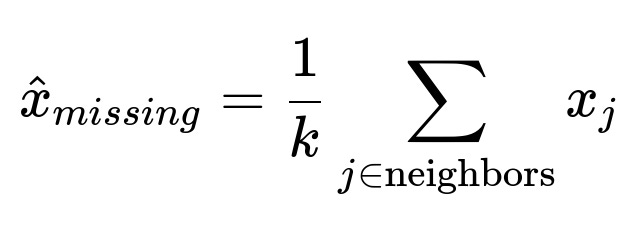
• For numerical features, we may take the mean of the neighbors.

• For categorical features, we may take the most common category among neighbors.

Pros

• Captures local structure in the data (assumes similar records are likely to have similar feature values).

• More flexible than simple mean/median approaches.

Cons

• Computationally expensive for large datasets, especially if repeated for many missing values.

• Highly susceptible to the curse of dimensionality, as distance metrics in high-dimensional spaces can become less meaningful.

• If data is missing for many features, the distance metric might be difficult to define.

Matrix Factorization Matrix factorization methods, such as those used in collaborative filtering or dimensionality reduction (e.g., SVD-based approaches), can predict missing entries by factoring the data matrix into latent factors:

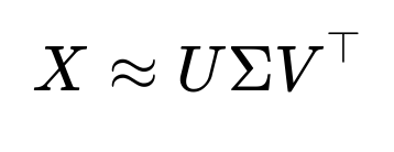
When we see missing entries, we can iteratively approximate them by fitting these low-rank factors. This is common in recommender systems (where user-item matrices have many missing entries) and can also be applied more generally.

Pros

• Can capture underlying low-rank structure, especially helpful if data is well-represented in a reduced-dimensional latent space.

• Can handle very large sparse matrices in specialized ways (like in big collaborative filtering systems).

Cons

• Requires iterative optimization methods and can be somewhat complicated to implement for small/medium tasks (though libraries exist).

• Assumes that the low-rank structure is a valid approximation of your data. If the data does not follow that assumption, the imputation might not be accurate.

Multiple Imputation (MICE)

Multiple Imputation by Chained Equations (MICE) is a technique where you iteratively impute missing values by fitting a series of models that “predict” the missing features using the other features. You do this multiple times to create multiple “complete” datasets, run analyses or train your models on each, and then combine the results in a statistically principled way.

Trade-offs

• Statistically more robust: It captures the uncertainty around missingness by producing multiple imputed values rather than a single guess.

• Computationally more expensive, because you train multiple models across multiple imputed datasets.

• Implementation complexity is higher, but it’s considered one of the more rigorous ways to handle missing data if you want to preserve variability and produce unbiased estimates.

Designing the Model to Handle Missing Indicators

Sometimes you can augment your dataset with a binary indicator variable that flags whether the value in a feature was missing. This approach can be especially useful in situations where the fact that a value is missing might itself be informative (for instance, a missing value can be systematically non-random).

In neural network contexts, it’s also possible to build architectures or use masked layers specifically designed to handle missing values (e.g., by ignoring them or learning embeddings for “missing” tokens for each feature).

Trade-offs

• It provides a direct signal to the model that a feature is missing, allowing the model to learn whether missingness correlates with the target.

• Can lead to more complex models or increased dimensionality (you add additional features as indicators).

• If data is MCAR, the indicator might add little value, but if data is missing not at random (MNAR), these indicators can be extremely helpful.

Bias and Missing Data Mechanisms

Data might be:

• Missing Completely at Random (MCAR): The fact that data is missing is independent of both observed and unobserved data.

• Missing at Random (MAR): The fact that data is missing depends only on observed data, not on the unobserved data.

• Missing Not at Random (MNAR): The fact that data is missing depends on unobserved data. For example, patients with higher severity of an illness are more likely not to report their symptoms.

Understanding these mechanisms helps you decide which imputation methods or dropping strategies might be acceptable or might introduce heavy bias.

Practical Example: Simple Imputation in Python

Below is a small snippet that uses scikit-learn’s SimpleImputer or KNNImputer:

import numpy as np
import pandas as pd
from sklearn.impute import SimpleImputer, KNNImputer

# Suppose we have a small numeric dataframe
data = {
    'feature1': [1.0, 2.0, np.nan, 4.0, 5.0],
    'feature2': [5.0, np.nan, 2.0, 1.0, np.nan],
    'target':    [0, 1, 0, 1, 1]
}

df = pd.DataFrame(data)

# Simple mean imputation
simple_imputer = SimpleImputer(strategy='mean')
df_imputed_simple = df.copy()
df_imputed_simple[] = simple_imputer.fit_transform(df[])

# KNN imputation
knn_imputer = KNNImputer(n_neighbors=2)
df_imputed_knn = df.copy()
df_imputed_knn[] = knn_imputer.fit_transform(df[])

print("Original:\n", df)
print("\nMean-imputed:\n", df_imputed_simple)
print("\nKNN-imputed:\n", df_imputed_knn)

In this example, SimpleImputer replaces missing values with the mean, while KNNImputer finds the closest neighbors (in terms of Euclidean distance by default) and imputes accordingly.

Conclusion of the Handling Strategies

• Dropping is straightforward but can lead to data loss and bias.

• Simple Imputation (mean/median/mode) is easy but can distort distributions and reduce variance.

• Advanced Methods like KNN or matrix factorization capture more structure but can be computationally expensive and require careful parameter tuning.

• Multiple Imputation provides a more statistically rigorous approach, at the cost of complexity.

• Modeling Missingness (missing indicators or specialized architectures) is particularly powerful when missingness itself carries information.

These choices often involve a trade-off between complexity, computational overhead, interpretability, and the risk of introducing or exacerbating bias. In an enterprise environment, you also consider ease of maintenance and reproducibility.

Below are potential follow-up questions with detailed discussions that might arise in a FANG interview context.

What if the proportion of missing data is extremely high? Would you still attempt imputation or might you engineer an entirely different approach?

When the proportion of missing data for a certain feature or set of features is extremely high, you have to be mindful of whether you are truly recovering meaningful signal from the small set of available non-missing data.

If the missing rate is very high on a feature (e.g., 90% of values are missing), you might:

• Drop the feature entirely, especially if it does not correlate strongly with your target.

• Investigate whether the pattern of missingness is itself predictive. In that case, you might keep the feature but rely heavily on “missingness indicators.”

• Use domain knowledge to see if that feature can be replaced by a proxy variable that is more reliably observed.

When the entire dataset is missing in many places (e.g., it’s not just one or two features, but a large portion of the table is incomplete), sometimes you consider alternative data collection methods, external data sources, or domain-driven engineering. In many real-world problems, you might incorporate external signals or design a process that ensures better data capture. For instance, if you find that your e-commerce system fails to capture certain attributes for certain types of purchases, you might want to redesign your data pipeline or user flow rather than relying purely on advanced algorithmic methods for imputation.

The trade-off is that advanced imputation techniques become less reliable as the missing proportion grows large, because you have fewer “observed points” from which to learn the latent structure.

How do you systematically detect if data is missing not at random (MNAR), and how do you handle MNAR in practice?

In practice, detecting MNAR can be very challenging because it requires external knowledge or assumptions about why data might be missing. You often look for patterns in the observed data that correlate with missingness:

• Compare distributions of a feature among rows that have other features missing vs. rows that do not.

• Evaluate external variables that might explain why certain features are missing. For example, a patient might fail to show up for a test when their health is deteriorating.

If you suspect MNAR, you can:

• Collect more domain knowledge to confirm. Sometimes domain experts can give insight into whether missingness is related to, for example, “income” or “disease severity.”

• Use missing indicators so that your model can at least learn that “missingness” correlates with outcomes.

• Use specialized models that are robust to non-random missingness (certain Bayesian methods or data augmentation techniques might help).

Ultimately, MNAR is best addressed with domain-driven solutions because purely algorithmic approaches cannot guess the unobserved values if the reason for missingness is entirely entangled with the unobserved values themselves.

Could you explain how multiple imputation handles uncertainty about the missing values in more detail?

Multiple Imputation by Chained Equations (MICE) works by recognizing that a single “best guess” imputation does not reflect the uncertainty. Instead, you do the following (conceptually):

1. For each feature with missing values, you create an imputation model that predicts this feature from all other features.

2. You iteratively impute the missing values multiple times, each time adding a stochastic component (for instance, by sampling from a predictive distribution).

3. You end up with several “complete” datasets, each of which is plausible given the observed data.

4. You train or analyze your target model on each of these complete datasets.

5. You combine the results (e.g., averaging the predictions or combining the parameter estimates) using rules that account for both within-imputation variance and between-imputation variance.

This means if the feature is highly uncertain, you’ll see more variability in those multiple imputations. That variability is reflected when you combine the results, leading to broader confidence intervals or more conservative estimates.

What considerations should be made for deep learning models in particular when data is missing?

Deep learning models typically require numeric inputs with no NaN values. You have to transform missing values into a valid numeric representation or a mask. Considerations:

• Embedding the concept of “missing”: In many contexts, especially with categorical or text-based inputs, you might represent “missing” as a separate token or embedding. The network can learn an embedding vector for the “missing” category.

• Masking: Some architectures (like certain recurrent neural networks or attention-based models) can incorporate masking that ignores missing timesteps or positions.

• Indicator variables: A straightforward approach is to add an indicator variable for each feature, denoting whether it is missing. The original feature is imputed (e.g., with a default value like 0.0 or the mean), and the indicator helps the model learn that it’s actually “missing.”

• Autoencoder-based imputation: You can train an autoencoder to reconstruct the data from partial observations. The hidden representation might learn how to fill in the blanks.

One must be mindful of the cost and complexity. For large-scale data with many missing values, a carefully designed approach or specialized library might be necessary.

How might you validate the effectiveness of an imputation strategy?

Validation of imputation typically involves:

• Synthetic experiments: Intentionally remove known values from the dataset, apply your imputation strategy, and compare the imputed values to the real values you removed. This helps measure how close your imputed values are to the actual values.

• Downstream task performance: The ultimate measure is often how well your model performs on a hold-out set or via cross-validation. If performance improves after employing a certain imputation method (compared to a baseline or simpler method), that suggests the approach is beneficial.

• Statistical properties: Check how well the imputation preserves means, variances, or correlations among features. If it severely distorts these relationships, it might bias your training.

How do you handle missing data during inference or deployment?

At inference time (or in production), missing data is often unavoidable. Your approach must be consistent with how you handled it at training time. For example:

• If you used mean imputation during training, you should continue to use the same mean value (calculated from the training set) to fill missing values at inference.

• If you used KNN imputation, you must either store the training data or the necessary statistics (though KNN typically requires the entire training dataset for distance calculations, which can be expensive). Alternatively, you might store cluster centers or a model specifically for imputation.

• If you used missing indicators, you must ensure those indicators are also provided at inference.

The key is that the data preprocessing pipeline used during training must be applied identically at inference. Mismatches in preprocessing or imputation can lead to degraded performance.

How do you decide between simple, advanced, or model-based imputation methods in a practical setting?

You consider:

• Data Size: If you have a massive dataset, advanced methods such as KNN can be expensive. Large datasets might also benefit from partial, distributed training solutions.

• Complexity vs. Gains: If simple mean or median imputation yields acceptable performance, you might prefer that over advanced methods for ease of deployment. However, if advanced imputation significantly boosts performance or fairness, you invest in it.

• Domain Knowledge: The domain might heavily inform you that certain features cannot be missing for certain reasons, or that the missingness has particular meaning.

• Time Constraints: KNN or matrix factorization might be more computationally intensive and might not scale in real-time systems.

• Fairness and Bias: Some regulatory or ethical contexts require a demonstration that your missing data handling does not systematically disadvantage certain groups. MICE or advanced modeling might offer more robust solutions.

Under what circumstances might you keep missing values as “unknown” categories without any imputation?

If you have categorical features with a possible “Unknown” or “Not Provided” category, it might be informative to keep missing data explicitly as an additional category. This can be meaningful in domains such as:

• Surveys, where skipping a question may indicate privacy concerns or a certain attitude.

• Observational data, where not reporting a value (like income) might correlate with another variable.

By doing so, the model can treat “Unknown” as a valid category. This approach is akin to adding an indicator for missingness but keeps everything in the same “one-hot” or embedding structure. You must be sure the “Unknown” or “Missing” category does not become overly conflated with other actual categories if your data pipeline is not carefully designed.

When might dropping records be a perfectly acceptable approach?

Dropping records is acceptable when:

• The percentage of missing values is very small, and the data is missing completely at random.

• The cost of losing those records is offset by the simplicity gains (e.g., if you have millions of data points and only 0.5% have missing entries in a particular feature).

• The records are known to be corrupted or otherwise unusable.

Even so, it’s typically good practice to check for patterns in the dropped data to ensure no systematic bias is introduced.

How do you handle missing data that appears only in the target variable?

When the target is missing, you typically cannot use that data point for supervised learning because you do not know the label. In some scenarios, you can:

• Use semi-supervised learning if you have partial labels.

• Use multiple imputation approaches that attempt to infer the target (though that might bias the training, as you’re guessing labels).

• Exclude those rows for the purpose of supervised training but still potentially use them in unsupervised or semi-supervised pretraining.

If your problem is classification or regression, you generally need the label to train. Missing labels effectively reduce the size of your labeled dataset. You might run separate pipelines for these “unlabeled” samples if you are considering semi-supervised or self-supervised approaches.

Does handling missing data differ between training deep learning models and traditional machine learning models?

The fundamental principles are the same—data is missing, and you need to handle it. However, deep learning typically:

• Requires numerical input without NaNs.

• Might have specialized layers for masking or embedding missing features.

• In practice, large neural networks can degrade if fed large amounts of artificially imputed data that differs significantly from the real distribution.

Traditional machine learning approaches (like XGBoost or random forests) can often handle missing data by splitting on “is missing” or by ignoring missing features, although typical implementations still require some form of imputation. The main difference is that deep learning frameworks require you to be very explicit about how you handle missing inputs.

What is the effect of outliers on imputation, and how do you handle them in conjunction with missing values?

Outliers can skew simple imputation methods (e.g., mean imputation heavily influenced by extreme outliers). You might:

• Use median instead of mean if the data is skewed or has outliers.

• Apply robust scaling or transformations (like log transforms) to reduce the impact of outliers before imputation.

• Use advanced imputation methods that are less sensitive to outliers or model-based approaches (e.g., robust regression in a MICE pipeline).

In general, it’s advisable to treat or investigate outliers separately. If your outliers are due to data entry errors, you might remove or correct them. If they are true extremes, you might keep them but use robust imputation.

Could you discuss some domain-specific examples where missing data handling is critical and might require specialized methods?

Healthcare

• Medical records are replete with missing labs or vitals. Missingness might be correlated with disease severity or patient adherence to treatment. In this case, advanced methods or missingness indicators can be vital to avoid systematic bias against severely ill patients who have incomplete records.

Finance

• Transaction data might have missing or delayed records due to system errors or user actions. Missing data in credit applications might correspond to risk levels. Proper handling or using missingness as a feature is important to avoid discriminatory lending practices.

Recommender Systems

• User-item matrices are mostly missing because users do not rate most items. Techniques like matrix factorization are standard. The missingness is typically not random; users only rate things they care about.

Sensor Networks

• Sensors might fail intermittently or have calibration errors. Time-based methods (forward/backward fill) or advanced spatio-temporal approaches that leverage neighboring sensors in a network can be used.

In all these domains, you must carefully reason about the nature of missingness. The techniques used can significantly impact fairness, interpretability, and model accuracy.

---

Below are additional follow-up questions

How do feature interactions complicate missing data handling, and what strategies ensure that imputed values do not disrupt interaction terms?

When features interact (for example, feature A times feature B in a polynomial expansion or cross term), missing values in one feature can invalidate direct interaction computations. If you impute them without consideration of the other interacting features, you risk introducing spurious correlations or losing important relationships.

One strategy to ensure that imputation does not disrupt interaction terms is to consider interaction features when imputing. For instance, if the interaction between two features is crucial for your model, you may:

• Use an imputation model that explicitly includes other features (and their interactions) as predictors.

• Incorporate domain knowledge: if you know feature A and feature B typically rise or fall together, a model-based imputation that includes both features will better preserve their joint distribution.

• Leverage advanced techniques such as Multiple Imputation by Chained Equations (MICE) where each feature can have a regression model that considers other relevant predictors. For interaction terms specifically, you might include the product term as a predictor in the chain, assuming you have some approximation for the missing part.

One subtle pitfall is that if interaction terms have high missingness in one or both features, naive single-value imputation might produce uniform (or near-uniform) interaction values that distort variance. This can lead to overly smoothed predictions. Another pitfall is overfitting if you try to model interactions in the imputation process without sufficient data, especially if the missing data is large in proportion. You can mitigate this by performing robust cross-validation, ensuring that the interaction-based imputation does not introduce artificial predictive power.

In high-cardinality categorical features, how can missing data be imputed without inflating the dimensionality or diluting important categories?

High-cardinality categorical features can have hundreds or thousands of unique categories, making traditional one-hot encoding unwieldy. If missing data exists for such features, one must consider:

• Category Grouping or Target Encoding: Instead of one-hot encoding, you might group categories with small counts into an “Other” category or use target encoding (averaging the target variable for each category) so that missing data can be imputed as the target average or some variant.

• Learnable Embeddings: In deep learning contexts, each category (including a special “missing” or “unknown” category) can have its own embedding vector. If a value is missing, you can map it to a special embedding that the network learns. This avoids huge sparse vectors.

• Imputation with Frequent Category or Probability Distribution: If the data is missing completely at random, a straightforward approach might be to assign the missing value to the most frequent category or to sample from the empirical distribution of observed categories. Sampling can preserve some variability but can also introduce noise.

• Pitfalls:

  • If you use target encoding, you risk data leakage if you compute the target-mean from the full dataset, including rows in your validation or test sets. The solution is to use out-of-fold or cross-validation strategies to ensure the target encoding is learned only on training folds.

  • If many categories are truly distinct in meaning, grouping them might lose some nuance, but if you do not group them, you risk an extremely large embedding or one-hot dimension. Balancing these trade-offs requires both domain knowledge and empirical testing.

  • “Missing” might itself be correlated with certain categories. If certain categories are more likely to be missing, you might need an extra indicator variable or separate embedding for “missingness.”

How might real-time data streams (e.g., streaming IoT sensor data) handle missingness on-the-fly without retraining a full imputation model?

When data arrives in real time—for example, from IoT sensors that sporadically lose connection—missing data must be handled quickly, often without time for complex offline retraining. Possible approaches:

• Rolling Averages or Exponential Smoothing: For numerical sensor values, you can maintain a rolling window of recent observations and fill the missing point with a short-term average or exponentially weighted moving average. This is a simple time-series approach that updates quickly.

• Online KNN or Incremental Models: Traditional KNN can be adapted to an online setting where you store recent samples in a buffer. If a new sensor reading is missing, you look up the nearest neighbors in your buffer. This can be resource-intensive but feasible if the buffer is kept small or if you use dimension reduction.

• Model-Based Prediction: You might train a lightweight online regression model on the sensor data (including other correlated sensors) and update its parameters incrementally. The model’s prediction for a missing sensor at time t can be used as the imputed value. If it’s a streaming random forest, you can maintain partial fits.

• Pitfalls:

  • Computational overhead in real time. Some advanced imputation techniques are too slow if you need millisecond-level latency.

  • Concept drift in sensor data. If the process changes over time, historical distributions might not apply anymore. An older model or imputation scheme might systematically bias the newly missing data.

  • Memory constraints. Storing large windows of historical data might be impossible, so you must be selective in how you keep track of the past (e.g., summarizing with statistics).

How do you handle missing data when feature importance or interpretability is a top priority, such as in regulated industries?

When working in highly regulated domains (healthcare, finance, insurance), interpretability is often paramount. The choice of imputation and how you handle missing data must be transparent and justifiable. Strategies include:

• Transparent Simple Imputation: Mean or median imputation can be documented easily, is explainable, and can be replicated by auditors. Coupled with missing indicators, this method ensures the model “knows” which values were imputed.

• Rule-Based Imputation: Domain experts might have specific rules for imputing or classifying missing data. For instance, “If the blood test is missing, check the patient’s last known stable reading. If that was within a normal range, use it; otherwise label as ‘missing unknown.’” This may be more transparent than purely data-driven solutions.

• Non-Complex Surrogate Models: If advanced techniques are needed, such as random forests or gradient boosting, you might keep them at a level that is still interpretable through feature importances or partial dependence plots. Complex deep learning with large embeddings might be harder to interpret unless you provide local interpretation methods.

• Pitfalls:

  • Overly simplistic imputation can degrade accuracy if the domain is complex.

  • Very detailed domain-based rules might become too rigid and fail in edge cases.

  • Regulators often demand consistency: you must prove that the same approach to imputation is used in production and yields consistent results. Any discrepancy can lead to compliance failures.

How can you handle missing data in multi-modal datasets, where some features are images, others are text, and still others are tabular?

Multi-modal datasets combine different data types, and each modality can suffer from distinct patterns of missingness. For instance, you might have an image from an MRI that is unreadable, a textual description that is partially filled out, and tabular clinical data with numeric features.

• Separate Pipeline per Modality: Often you build separate encoders—such as a CNN for images, an RNN or transformer for text, and a standard feed-forward net for tabular data—and then fuse these representations. Each encoder can handle missingness specific to its domain. A textual encoder can treat missing text as an “empty string” or “unknown token,” while an image encoder can handle partial or corrupted images with in-painting or masked convolution.

• Cross-Modal Imputation: If the missing data in one modality can be inferred from another, you might use cross-modal attention or gating. For example, the textual description might fill in details about the patient’s condition that are missing from the numeric tabular data. However, this typically requires advanced neural architectures that can fuse incomplete embeddings from each modality.

• Pitfalls:

  • Some domains may be missing entire modalities for a subset of samples (e.g., some patients don’t have MRI scans at all). If that subset is large, the model might not properly learn cross-modal relationships.

  • Complex multi-modal models can be expensive, making real-time inference and real-time imputation difficult.

  • Overfitting can occur if the model tries to “guess” too precisely from partial signals in other modalities without truly robust data. Thorough cross-validation is necessary to ensure generalization.

How do you adapt missing data handling strategies for large-scale distributed systems, such as Spark or Hadoop clusters?

When working on distributed systems with very large datasets:

• Distributed Simple Imputation: You can compute global statistics (mean, median) in a distributed manner (e.g., using Spark’s aggregate operations). This is straightforward but might ignore local data patterns if the dataset is heterogeneous across nodes.

• KNN or MICE at Scale: KNN typically does not scale well in high dimension or with huge datasets. You might employ approximate nearest neighbor search or sample subsets of data. MICE can be parallelized by distributing the imputation of each feature across different workers, but it can still be quite heavy computationally.

• Incremental or Streaming Factorization: Matrix factorization methods like ALS (Alternating Least Squares) are often implemented in Spark for recommendation systems. These can handle missing entries in a distributed setting.

• Pitfalls:

  • Network overhead. Collecting partial data across many nodes to perform a global imputation can be bottlenecked by data shuffles.

  • Inconsistent partial aggregates. If the data splits are highly imbalanced, a global mean might not represent any single subset well. A hierarchical approach might be used, computing local means on each partition and then a second-level mean across partitions.

  • Versioning and reproducibility. You must track which version of the dataset had which imputation, especially if your pipeline processes data in micro-batches or near real-time.

How to handle missing data in unsupervised learning or clustering tasks, where there is no target variable?

In unsupervised tasks (like clustering or density estimation), the notion of “performance” is less tied to a predictive outcome, so missing data handling must rely on the internal structure of the data itself.

• Pairwise Distance Measures: Some clustering algorithms (like hierarchical clustering) allow you to define a custom distance metric that ignores missing features or penalizes them in specific ways. This can be more natural than forcing an imputation.

• Imputation via Dimensionality Reduction: Techniques like PCA can be adapted to handle missing values by using iterative approaches that fill missing entries with the low-rank approximation. This is somewhat related to matrix factorization.

• Soft Clustering: Mixture models (e.g., Gaussian Mixture Models) can be extended to handle missing data by marginalizing over the missing dimensions if the distribution is assumed. This requires an expectation-maximization (EM) approach that iteratively estimates missing values.

• Pitfalls:

  • If you choose a distance metric that simply ignores missing dimensions, it might produce inflated distances if many features are missing.

  • EM-based approaches can converge to local minima or become unstable if too many values are missing.

  • In purely unsupervised settings, it’s harder to validate whether an imputation strategy is “correct,” since you don’t have labels to measure performance. One typically relies on metrics like silhouette scores or domain interpretability to judge the coherence of clusters.

How does the severity of multicollinearity among features affect your missing data imputation strategy?

When features are highly correlated (multicollinearity), certain advanced imputation methods can become unstable or redundant:

• Benefits: If features are strongly correlated, imputation might be more accurate because the model can use correlated features to predict the missing values of another. Techniques like MICE or regression-based imputation can exploit collinearity to fill in missing entries more effectively.

• Pitfalls:

  • Overfitting: If two features are almost identical, imputation by regression might incorrectly produce perfect or near-perfect fills during training, leading to unrealistic performance estimates in cross-validation.

  • Inverse matrix operations (in linear or logistic regression-based imputation) can be numerically unstable if collinearity is very high. You might need regularization techniques (like ridge or lasso) to handle that.

  • If the collinearity is domain-driven (e.g., two sensors measuring similar phenomena), you might question whether you need both features in the first place or if dropping one feature can simplify the pipeline.

• Practical Approaches:

  • Introduce mild regularization in your imputation models.

  • Consider principal component analysis to reduce dimensionality before performing simpler imputation on a reduced set of principal components. Then transform back if needed.

  • Carefully validate using cross-validation that includes the imputation step inside each fold to avoid overly optimistic results.

What steps can be taken to ensure fairness and mitigate potential disparate impact when different demographic groups have different rates of missingness?

If certain demographics or protected groups systematically have more missing data (e.g., lower-income individuals less likely to fill out certain forms), naive imputation might cause biased model predictions. Steps to ensure fairness include:

• Stratified Analysis: Perform missingness analysis by subgroup to detect if one group has a higher proportion of missing values.

• Fairness-Aware Imputation: Incorporate group or demographic information as part of the imputation process, ensuring the algorithm does not systematically bias imputations for one group. However, you have to be mindful of privacy concerns if you explicitly use protected attributes.

• Separate Models: In extreme cases, you might train separate imputation models for each demographic group if that yields more accurate and fair imputations. This can also be done if domain knowledge suggests that each group’s data generating process is different.

• Monitoring Metrics: Use fairness metrics (e.g., demographic parity, equal opportunity) on the final model predictions. If discrepancies exist, investigate whether the cause is related to how missing data was imputed.

• Pitfalls:

  • Using protected attributes in the imputation pipeline might have regulatory implications. Some laws and guidelines discourage or restrict the use of sensitive attributes in modeling.

  • Treating each group separately can reduce sample size for each subgroup, possibly leading to less robust imputations.

  • Fairness is multi-faceted. Eliminating disparities in one metric might increase them in another, so you need broad stakeholder agreement on fairness definitions.

When might you consider entirely discarding the concept of imputation and designing a model that natively handles missingness?

Some model classes, like certain tree-based methods, can handle missingness to a degree without explicit imputation. Examples:

• Decision Trees: Some implementations let you split on “is feature X missing?” or have a separate branch for missing values. This way, missingness is handled as a natural category without substituting a numeric or categorical placeholder.

• Neural Network Approaches with Masking: You can pass in a mask tensor indicating which values are present or missing, and the architecture can skip or adapt the computations for missing elements.

• Pitfalls:

  • Not all libraries or frameworks implement missingness in a robust manner. Some require explicit numeric filling.

  • If the distribution of missing values is large or highly non-random, a specialized approach might still be needed.

  • Interpretability can be more challenging because you have to explain how the model deals with missingness in real-time.

In certain cutting-edge scenarios (like large language models that process textual descriptions), you might incorporate missingness by simply not including data or by specifying placeholders in the text. The model’s architecture (transformers with attention) might be able to adapt. This discards the need for a separate imputation step entirely, but you must confirm that performance meets your requirements and that you’re not introducing subtle biases by ignoring missingness patterns.

How do you ensure data integrity and reproducibility when different teams or pipelines might apply different imputation methods over time?

In many organizations, data pipelines evolve, and different teams might apply different transformations or updates to the same dataset. This can lead to inconsistencies. Best practices to ensure reproducibility:

• Centralized Data Dictionary and Pipeline: Document the exact imputation steps. For instance, specify that “Feature A is imputed with the median value from the 2021 training set,” and store that median.

• Version Control for Data: Just like code, you can version the dataset or the transformation code. Tools like DVC (Data Version Control) or MLflow can store metadata about how imputation was performed and with which parameters.

• Automated Deployment: The same pipeline code (e.g., a Python module) is used for both training and inference. This ensures consistent transformations.

• Pitfalls:

  • If multiple teams try to replicate your pipeline but use slightly different techniques or a different subset of data to compute the imputation statistics, results can diverge.

  • Over time, new data may shift the distribution of features, so the original median from 2021 might no longer be relevant. You must decide whether to periodically refresh the imputation parameters.

  • If you are in a regulated environment, an auditor might question any changes to how imputation is done, so you need thorough change logs and justification.

In what scenarios might it be appropriate to systematically incorporate expert rules or external data sources to fill in missing values rather than relying on purely data-driven imputation?

Sometimes domain knowledge or external reference databases are more reliable than the data you have. Examples:

• Healthcare: If a patient’s lab value is missing, you might have an official health registry that tracks historical lab results for the same patient at a different clinic. Or a domain rule might say, “If X lab test is missing but the patient’s vital signs are stable, assume a normal range unless certain symptoms are present.”

• Geographic Data: Missing location data might be enriched from external mapping services (e.g., if the street name is missing, but you have the zip code and city).

• Financial Data: If the credit score is missing, you can query external credit bureaus.

• Pitfalls:

  • Integrating external data can be costly, time-consuming, and might require additional privacy or compliance checks.

  • The external source could also have missing or outdated information.

  • Domain-specific rules might be heuristic and not always accurate, introducing systematic bias or overshadowing patterns the model might learn from the raw data.

How do you handle missingness for ordinal features (where data is categorical but has a natural order)?

Ordinal features, such as “low,” “medium,” “high,” or “stage 1,” “stage 2,” “stage 3,” have an inherent ranking. If there are missing values, simple mode or median-based methods can ignore that ordering:

• Ordinal Encoding: Convert categories to numeric ranks (e.g., “low”=1, “medium”=2, “high”=3). Then you can apply numeric imputation methods like mean or median. But be cautious: for ordinal data, the mean might not represent a permissible category. Instead, you might round to the nearest integer rank.

• Domain-Driven Imputation: If you have partial knowledge, like “it’s definitely not ‘low,’ but we don’t know if it’s ‘medium’ or ‘high,’” you might want a specialized approach that picks from a restricted set. Or you might assign a distribution across the plausible categories.

• Pitfalls:

  • If you treat ordinal data as purely numeric, you might incorrectly treat the distance between “low” and “medium” as the same as between “medium” and “high.”

  • If the missing rate is high, you might lose the ordinal structure because the model sees too many placeholders.

  • Overly simplistic approaches can degrade the subtlety in ordinal data, especially if the categories are broad and the difference between them is clinically or practically significant.

Can adaptive methods like active learning or experiment design reduce missingness for critical features in future data collection?

Active learning or adaptive experiment design can be used to proactively reduce missing data for important features, especially if acquiring that feature has a cost or logistic constraint.

• Active Feature Acquisition: Instead of always collecting every feature from every instance (which might be impossible or too expensive), a system can decide which features are most valuable to measure. For high-value data points (e.g., uncertain predictions, critical patients), the system might prompt for additional testing or attempt to fill missing data by specifically requesting that information.

• Example: A healthcare triage system might request certain lab tests if it’s uncertain about a patient’s status, thereby actively reducing missingness for crucial features over time.

• Pitfalls:

  • Implementation complexity. Actively designing experiments or deciding which features to measure in real time requires specialized infrastructure and potential domain permissions.

  • Bias if the system only requests data for borderline or uncertain cases, leaving out the majority of “certain” cases, which can lead to skewed overall distributions.

  • Cost-benefit trade-off. If certain features are expensive or time-consuming to collect, you need to justify the additional cost based on improved model performance or safety considerations.

How might domain knowledge about the probability distribution of a feature guide the choice of imputation?

If you have strong prior knowledge about how a feature is distributed—maybe it follows a log-normal distribution or a beta distribution constrained between 0 and 1—this can guide your imputation:

• Parameter Estimation: Estimate the parameters of the distribution (like mean and variance for a normal, or shape parameters for a beta). Then sample missing values from that fitted distribution, preserving variance and shape.

• Bayesian Approaches: You can use prior distributions for the parameters, and the observed data updates your beliefs via a posterior distribution. Missing values can then be sampled from the posterior predictive distribution, naturally reflecting uncertainty.

• Pitfalls:

  • Incorrect distribution assumptions can lead to systematically biased imputations.

  • Parametric approaches can break if the observed data has heavy tails, outliers, or multi-modal structure not captured by the chosen distribution.

  • If the domain knowledge is incomplete or partially incorrect, your final results might degrade overall model performance despite best intentions.