ML Interview Q Series: How are K-Nearest Neighbors and Support Vector Machines different in their fundamental methods, and when might one approach surpass the other?

📚 Browse the full ML Interview series here.

Comprehensive Explanation

K-Nearest Neighbors (KNN) and Support Vector Machines (SVM) both tackle classification (and sometimes regression) tasks, but they approach the problem in distinctly different ways, with varying trade-offs in terms of training speed, inference speed, interpretability, and performance on certain types of data.

Understanding K-Nearest Neighbors

KNN is often referred to as a “lazy learner.” There is essentially no explicit training step: it stores the training data and waits until a new example arrives for classification. When a new data point is presented, KNN will look at the k closest points (according to some distance metric) in the training set and use those neighbors to determine the class of the new data.

The most common distance metric used in KNN is Euclidean distance, typically computed as a square root of the sum of squared differences across each feature dimension. For example, in text-based format for two points x and y in an n-dimensional space, the Euclidean distance can be represented as:

distance = sqrt( (x1 - y1)^2 + (x2 - y2)^2 + ... + (xn - yn)^2 )

Choosing an appropriate distance metric is crucial. Euclidean distance is common, but for text-based or high-dimensional data, other metrics like Manhattan distance or cosine similarity may be used.

Main Characteristics of KNN

KNN is usually straightforward to implement and interpret. However, it can become computationally expensive at inference time because the model must search the entire dataset (or large subsets of it) to find the closest neighbors. Efficient search structures like KD-trees or Ball Trees can help mitigate some of these costs, but KNN often remains less suitable for extremely large datasets, especially in high dimensions.

Another key consideration is that KNN’s performance depends on choosing an optimal value for k. A small k can lead to overfitting, while a large k can lead to underfitting or oversmoothing the decision boundary.

Understanding Support Vector Machines

SVM is a discriminative classifier that focuses on finding an optimal hyperplane (or set of hyperplanes) in a high-dimensional space that can separate data points belonging to different classes. It tries to maximize the margin between the classes, leading to robust boundaries that can generalize well.

A key concept in SVM is the margin: the distance from the separating hyperplane to the closest training data points (the support vectors). By maximizing this margin, SVM tries to reduce overfitting and improve the model’s capacity to generalize.

SVM can also handle non-linear classification by using the “kernel trick.” Common kernels include the polynomial kernel and the Gaussian Radial Basis Function (RBF) kernel. These kernels implicitly map data into a higher-dimensional feature space, allowing SVM to find non-linear boundaries in the original input space.

Below is a standard expression for the hinge loss, which is at the core of the SVM optimization problem. The goal of the SVM is to minimize this loss while maximizing the margin:

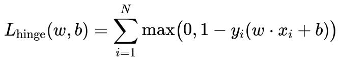
Where:

• w is the weight vector of the SVM hyperplane in the feature space.

• b is the bias term (the intercept).

• x_{i} is the i-th data point.

• y_{i} is the label of the i-th data point, typically +1 or -1.

• N is the total number of training examples.

The SVM solution also includes a regularization component that balances margin maximization with ensuring we do not over-penalize misclassifications in the presence of noise.

Main Characteristics of SVM

When feature space is large, SVM (especially with an appropriate kernel) often performs well. It has a strong theoretical foundation, guaranteeing good generalization if its parameters (e.g., kernel parameters, regularization parameter C) are well-chosen. SVM can be more complex to implement from scratch compared to KNN, but many efficient libraries exist to handle training on diverse data types. However, as the dataset grows very large, the training time of SVM can become considerable, particularly if you use kernelized SVM with complex kernels.

Contrasting KNN and SVM

KNN does not have a real training phase, so it is fast to “train,” but can be slow to predict. It also lacks interpretability when data grows large, and performance can degrade in high-dimensional feature spaces if distance metrics become less meaningful.

SVM is a more structured, model-based approach that tries to find an optimal boundary. Once trained, predictions are typically fast because classification only depends on computing an inner product between the test point and a subset of support vectors. However, SVM might need more careful tuning (kernel selection and parameter tuning) and may take longer to train on large datasets.

KNN is often preferred in cases where the data is reasonably small or can be indexed efficiently, and where local structure is highly meaningful. SVM may outperform KNN when the data has well-defined margins or is separable (linearly or with kernel transformations), especially in moderate-to-high dimensional spaces with carefully chosen kernel functions.

Practical Python Code Examples

Below is a simple Python example demonstrating how you might train an SVM classifier using scikit-learn.

from sklearn.svm import SVC
from sklearn.metrics import accuracy_score
from sklearn.model_selection import train_test_split

# Suppose X, y are your data and labels
X_train, X_test, y_train, y_test = train_test_split(X, y, test_size=0.2, random_state=42)

svm_model = SVC(kernel='linear', C=1.0)
svm_model.fit(X_train, y_train)

predictions_svm = svm_model.predict(X_test)
accuracy_svm = accuracy_score(y_test, predictions_svm)
print("SVM Accuracy:", accuracy_svm)

And an example for KNN:

from sklearn.neighbors import KNeighborsClassifier
from sklearn.metrics import accuracy_score
from sklearn.model_selection import train_test_split

# Suppose X, y are your data and labels
X_train, X_test, y_train, y_test = train_test_split(X, y, test_size=0.2, random_state=42)

knn_model = KNeighborsClassifier(n_neighbors=5)
knn_model.fit(X_train, y_train)

predictions_knn = knn_model.predict(X_test)
accuracy_knn = accuracy_score(y_test, predictions_knn)
print("KNN Accuracy:", accuracy_knn)

What to Keep in Mind

Hyperparameter selection is important for both algorithms. For KNN, selecting k has a significant effect on bias-variance. For SVM, the choice of the kernel function and regularization parameter can change the decision boundary dramatically. Preprocessing and feature scaling often improve results for both methods, especially for distance-based classifiers like KNN and margin-based methods like SVM.

How to Decide Between KNN and SVM

In domains where data points of the same class are naturally close to each other and the dataset is not too large, KNN can be a simple yet effective approach. On the other hand, if you suspect that there exists a clear margin (or margin in a transformed kernel space) separating the classes, and you can afford a more involved training phase, SVM may offer better generalization.

Follow-Up Questions

How does the dimensionality of the feature space affect KNN and SVM differently?

When the dimensionality of data increases, distance-based approaches like KNN may struggle because distances become less meaningful (“curse of dimensionality”). KNN can suffer significantly as the points tend to become equidistant, potentially decreasing the value of the nearest-neighbor concept. SVM can also be affected, but kernel-based methods sometimes mitigate high-dimensional challenges by mapping features into spaces where a separating hyperplane can still be found. Moreover, with proper regularization and careful kernel choice, SVM can handle moderately high dimensions more gracefully than a naive KNN approach. However, extreme dimensionality still poses challenges to SVM, particularly in terms of computational complexity and overfitting if the kernel parameters are not well-tuned.

Can KNN handle noisy data effectively compared to SVM?

KNN can be quite sensitive to noise because a single outlier point close to a test sample can dominate the voting if k is small. Increasing k can reduce the effect of outliers, but it can also over-smooth boundaries. SVM, especially in its soft-margin formulation, can handle noisy data by allowing certain misclassifications but penalizing them to find a balance between margin maximization and misclassification. This approach can be more robust to noise if hyperparameters (like the regularization parameter C) are properly tuned.

What happens if the classes are highly imbalanced?

KNN will have a tendency to classify new points into the majority class more frequently, particularly if k is large, since the majority class neighbors will dominate. One approach to mitigate this is to weigh neighbors by distance or apply other rebalancing strategies. SVM can also be sensitive to class imbalance, but there are strategies like class-weighted SVM or adjusting decision thresholds that can help. Both methods require careful calibration or cost-sensitive training approaches if the dataset is significantly skewed.

How does kernel selection in SVM compare to distance metric selection in KNN?

Both kernel selection in SVM and distance metric selection in KNN fundamentally affect the notion of similarity between data points. In KNN, choosing Euclidean, Manhattan, or another metric changes how neighbors are determined. In SVM, choosing a linear, polynomial, or RBF kernel changes the shape of the boundary and the way data is mapped to a higher-dimensional feature space. Both tasks often require empirical experimentation and domain knowledge. Proper cross-validation can guide selection, but it’s usually a process of iteratively testing and refining choices.

Why might model training and prediction speeds be relevant when choosing KNN or SVM?

KNN’s training time is negligible, since it merely stores the data. However, prediction time can be large, because for each query point the algorithm has to search the training set to find nearest neighbors. This can be a major disadvantage if you need real-time predictions and have a large dataset. SVM, by contrast, can have a comparatively larger training time. But once trained, the model uses only the support vectors for classification, making predictions generally fast. Therefore, if training time is not a bottleneck but prediction time is critical, SVM is often the more appropriate choice.

Are there any specific domains where KNN or SVM distinctly shine?

KNN is traditionally popular in recommendation systems, some medical applications (like disease classification based on patient proximity in feature space), and scenarios with smaller datasets. SVM is widely used in text classification, image recognition, and bioinformatics because of its strong theoretical guarantees and capacity to handle a variety of non-linear separations via kernels. However, deep learning methods have also encroached on areas where SVM was once dominant, so the choice nowadays might also include neural network models, depending on the dataset and task complexity.

Below are additional follow-up questions

How do we handle multi-class classification with both SVM and KNN?

When your dataset has more than two classes, you need to extend SVM (which fundamentally handles binary classification) to a multi-class scenario. Typical approaches include the “one-vs.-rest” strategy (training a separate classifier to distinguish one class from all others) and the “one-vs.-one” strategy (training a classifier for every pair of classes). In scikit-learn, these strategies are already abstracted away inside the implementation, so the user rarely has to manage them manually. However, each approach impacts training time and memory usage differently. For example, one-vs.-one for C classes involves training C*(C-1)/2 classifiers, which can become computationally expensive for large C.

On the KNN side, extending to multiple classes is more straightforward: you still vote among the nearest neighbors, but now those neighbors can belong to more than two classes. Whichever class receives the most votes is selected as the predicted class. Potential pitfalls include ties, where multiple classes might receive the same number of votes. Such ties can be resolved via distance weighting or random selection.

A subtle real-world edge case is highly imbalanced multi-class data where some classes have far fewer examples than others. The one-vs.-rest approach might struggle because the minority class can easily be overshadowed. Similarly, for KNN, minority-class samples may be too few or too far from each other, leading to incorrect predictions. Data augmentation or balancing strategies can help in such scenarios.

What are the memory usage considerations for KNN vs. SVM?

KNN is memory-intensive because it needs to store all or most of the training data. During inference, it scans the stored examples to determine nearest neighbors. For very large datasets, this becomes problematic, leading to high memory consumption and slower lookups. Advanced data structures like KD-trees or Ball Trees can partially mitigate these costs but can also have performance degradation as dimensionality increases.

SVM primarily stores the support vectors rather than the entire training set. Especially in cases where only a small fraction of training examples are support vectors, memory usage can be significantly lower than KNN. However, for certain kernels or high complexity data, many examples might end up as support vectors, limiting this advantage.

An edge case arises when you have streaming data: the dataset might grow continuously, and memory usage for KNN can blow up because you keep all historical data. SVM might handle streaming data better with incremental learning techniques or a limited set of support vectors, but specialized implementations are required.

How do we interpret the decision boundaries from SVM vs. the local decisions from KNN?

SVM, particularly in its linear form, creates a clear global decision boundary—a hyperplane that separates classes. This global boundary can be relatively straightforward to visualize and understand in lower-dimensional settings (e.g., 2D or 3D). In kernelized SVM, the boundary can be more complex, but it remains a global separation guided by support vectors.

KNN lacks an explicit global boundary. Instead, it decides classification based on local neighborhoods in the feature space. This often leads to highly irregular boundaries that can adapt flexibly to the data distribution but may be more difficult to interpret at a global level.

A subtlety arises when data contains localized regions that overlap or have different densities. KNN can potentially capture these local nuances well, but it also can produce overly fragmented boundaries if k is too small. With SVM, a global boundary can sometimes be too coarse if the data has many small “pockets” of classes, unless the kernel is tuned to capture those complexities.

How do SVM and KNN handle data with significantly overlapping classes?

When classes heavily overlap, it can be difficult to find a perfect separation for SVM—especially if you insist on a hard margin. A soft-margin SVM allows some misclassifications, balancing margin maximization against misclassification penalties. You can adjust the penalty parameter to trade off between fitting training data and avoiding overfitting.

For KNN, overlapping classes mean that the nearest neighbors might belong to multiple classes in close proximity. Smaller k values might lead to noisy boundaries, whereas larger k values might blur distinctions too much. Tuning k becomes critical, and sometimes a weighted-voting scheme (where neighbors are weighted inversely by their distance) can help.

An important real-world pitfall involves deciding how to label a new point that lies right in the heart of an overlapping region. Even small differences in hyperparameters (like SVM’s regularization parameter or KNN’s distance metric) can yield drastically different decisions. Visualizing the data and performing thorough cross-validation often helps reveal the extent of overlap and guides a suitable choice of hyperparameters.

Can KNN or SVM be adapted for streaming or incremental data scenarios?

Out of the box, KNN is not naturally suited to streaming data because it stores all examples. As new data streams in, you keep adding points, making both storage and query times grow. Some variants, like Nearest Neighbor with dynamic forgetting or prototype-based methods, attempt to select representative points and discard old ones.

SVM also typically requires batch training. However, online or incremental SVM methods do exist. They update the set of support vectors incrementally as new data arrives, removing or adjusting obsolete support vectors and introducing new ones as needed. These methods can still be computationally intensive, but they’re generally more memory efficient than naive KNN.

A real-world edge case is concept drift, where the data distribution changes over time. Models trained on older data become less relevant. Incremental approaches for both SVM and KNN must have a strategy to forget or discount outdated data. KNN might overweight older points if it stores them indefinitely, while an incremental SVM might have stale support vectors if they aren’t removed in a timely manner.

When deploying these models to production, how do you handle updates in data distribution for KNN vs. SVM?

In a production environment, data distributions can shift over time due to seasonality, user behavior changes, or external factors. For KNN, adding new data means storing more samples, which can degrade prediction speed and memory usage. One practical approach is to periodically retrain with a window of the most recent data rather than the entire historical dataset. Some practitioners also maintain smaller “centroids” for each local region, effectively compressing the data.

With SVM, you can either periodically retrain in a batch fashion on fresh data or use incremental/online SVM methods that adjust the support vectors as new data arrives. However, retraining from scratch can be computationally expensive for large datasets, and incremental methods can be complicated to implement correctly.

A subtle pitfall includes not properly monitoring data drift. If the distribution shifts significantly, both models can become less accurate if not retrained or updated. Also, newly emerging classes (or anomalies) might not be recognized. A robust deployment architecture should include monitoring of prediction performance, automated alerts when performance degrades, and a strategy for model refreshing or adaptation.