
ML Interview Q Series: How can a Confusion Matrix be leveraged to evaluate the quality of a classification model’s predictions?


📚 Browse the full ML Interview series here.
Comprehensive Explanation
A confusion matrix is a table-based representation used to evaluate the outcomes of a classifier. In the simplest binary classification setting, the matrix summarizes how many instances were predicted correctly or incorrectly across both the positive and negative classes. It helps visualize the counts of true positives, false positives, false negatives, and true negatives, which are essential for computing a variety of performance metrics.
Once you have the counts in the confusion matrix (TP, FP, TN, and FN), you can derive metrics such as accuracy, precision, recall (also called sensitivity), specificity, and the F1 score. These metrics guide you in evaluating different aspects of your model’s strengths and weaknesses. For instance, precision quantifies how reliable your positive predictions are, while recall tells you how many actual positives your model manages to capture.
Key Derived Metrics
Accuracy is one of the most common measures but can be misleading with imbalanced datasets. It is calculated as the proportion of correctly classified instances over the total number of instances. You can express it using the confusion matrix elements:

Precision specifies what fraction of predicted positives are truly positive. Recall specifies what fraction of actual positives are correctly identified:


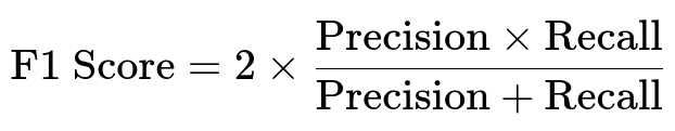
These two measures are combined into the F1 score, which provides a harmonic mean of precision and recall:
You typically choose precision or recall to optimize based on your specific use case. For example, in medical diagnostics you might prioritize recall to identify as many positive cases as possible, even if it means generating more false positives.
Practical Application in Different Scenarios
The utility of a confusion matrix extends to multi-class scenarios as well, but in that case the matrix grows to K x K for K classes, showing how often each class is being confused with others. This allows you to pinpoint where the model is making mistakes and which classes are particularly challenging to classify.
In highly imbalanced classification problems, accuracy can be misleading because the model can predict the majority class almost all the time and still achieve high accuracy. Instead, metrics derived from the confusion matrix, such as precision, recall, and the F1 score, are more robust indicators of performance in such cases. You can also track metrics like the ROC curve and precision-recall curve to better visualize performance trade-offs.
Code Illustration in Python
Below is a brief Python snippet to demonstrate how to compute and visualize a confusion matrix using scikit-learn:
import numpy as np
from sklearn.metrics import confusion_matrix

# True labels and predicted labels
y_true = [1, 0, 1, 1, 0, 0, 1]
y_pred = [1, 0, 1, 0, 0, 1, 1]

# Compute the confusion matrix
cm = confusion_matrix(y_true, y_pred)
print("Confusion Matrix:\n", cm)

# cm will be in the format:
# [[TN, FP],
#  [FN, TP]]
To visualize, you can use seaborn:
import seaborn as sns
import matplotlib.pyplot as plt

sns.heatmap(cm, annot=True, fmt="d", cmap="Blues")
plt.xlabel("Predicted")
plt.ylabel("Actual")
plt.show()
This gives you a heatmap indicating the counts for each cell (TN, FP, FN, TP).
Potential Pitfalls and Edge Cases
Sometimes it is easy to rely solely on accuracy or just one of the derived metrics. This can obscure the true predictive performance if the dataset is skewed toward one class. In certain domains like fraud detection or medical diagnosis, a small subset of the population is of high importance (positive cases), so focusing on recall or the F1 score is often more critical than simply maximizing accuracy.
If classes are imbalanced, you might also consider other techniques such as stratified sampling, over-sampling the minority class (e.g., SMOTE), or under-sampling the majority class to ensure your confusion matrix and metrics reflect the model’s performance fairly.
Follow-Up Questions
How do you handle multi-label classification scenarios with confusion matrices?
Multi-label classification involves predicting multiple labels simultaneously for each sample. In such cases, each label can have its own confusion matrix. You treat each label as a separate binary classification task, compute the confusion matrix for each label individually, and then aggregate metrics across all labels if needed. Alternatively, you can compute the average confusion matrix if you want an overall perspective, although that approach might lose label-specific performance nuances. It is often more insightful to look at each label’s confusion matrix to determine which labels are harder to predict.
Is the confusion matrix useful in regression tasks?
A confusion matrix is not applicable to regression, because regression predicts a continuous output and there are no discrete classes to compare against. For regression tasks, other error metrics such as mean squared error, mean absolute error, or R-squared are more appropriate.
Which metric is most critical to focus on if classes are highly imbalanced?
In highly imbalanced settings, metrics such as precision and recall, or their harmonic mean (the F1 score), become more informative. Recall is often prioritized if the cost of missing a positive is high (e.g., failing to detect a fraudulent transaction). Precision becomes paramount if false positives are very costly (e.g., an expensive medical procedure is triggered by a positive prediction). The choice depends on the real-world consequences of different error types.
How do you select a threshold for your predictions using the confusion matrix?
The confusion matrix can be recomputed at various thresholds if your classifier outputs probabilistic predictions. By adjusting the threshold from 0.0 to 1.0, you will produce different rates of true positives, false positives, and so forth. You select the threshold that strikes the best trade-off among metrics like precision, recall, F1 score, or a business-specific cost function. Visualization tools such as ROC curves or precision-recall curves assist in selecting the threshold that optimally balances these error types.
How do you expand the confusion matrix analysis for multi-class classification?
For multi-class problems, a K x K confusion matrix is formed, where K is the number of classes. The cell at row i and column j indicates how many samples of class i were predicted as class j. An examination of each row helps identify which classes the model is confusing with others. For example, if class 2 is often misclassified as class 3, you may need additional representative data or more targeted feature engineering to distinguish between those classes. You can compute metrics like precision, recall, and F1 on a per-class basis (often called micro- or macro-averaged metrics) to summarize performance across all classes.
Below are additional follow-up questions
Can a confusion matrix help in cost-sensitive scenarios, and if so, how?
Cost-sensitive scenarios arise when different misclassifications incur different penalties. For example, classifying a fraudulent transaction as legitimate might be significantly more costly than wrongly flagging a legitimate transaction as fraudulent. In these situations, you can extend the basic confusion matrix into a cost matrix, assigning a cost for each type of error. The aim is then to minimize the total misclassification cost rather than just error rates.
One practical approach is to use the confusion matrix to guide threshold tuning. Instead of strictly maximizing accuracy or F1 score, you modify your decision threshold based on the relative costs of false positives and false negatives. If the cost of a false negative is substantially higher, you may lower the threshold to reduce the chance of missing a positive. When the model predicts probabilities, you can iterate over possible thresholds, each time computing the cost-adjusted metric derived from the confusion matrix, and choose the threshold that minimizes the overall cost.
Pitfalls:
If the cost matrix is not representative of real-world conditions, or if the costs are oversimplified, you might tune your model incorrectly.
Real-life costs can be dynamic (e.g., the cost of missing fraud may change depending on seasonal or behavioral factors), requiring continuous re-evaluation of the cost matrix.
How do you manage a confusion matrix when there are many classes?
When the classification problem involves a large number of classes (sometimes hundreds or thousands), the confusion matrix becomes very large (K x K, where K is the number of classes). Visualizing it can be unwieldy, and spotting performance issues by mere inspection is challenging.
You can manage this complexity by:
Grouping similar classes into broad categories to get a high-level view. For instance, if you have multiple classes that belong to the same broader category, you might aggregate them to see general confusion patterns at a category level.
Focusing on top misclassified pairs. Often, certain classes are frequently mistaken for one another. By identifying these pairs, you can focus improvement efforts where they have the largest impact.
Computing per-class precision and recall (or F1 score), then comparing these metrics across classes. This helps pinpoint which classes perform significantly worse.
Pitfalls:
If certain classes are rarely observed, the corresponding rows or columns in the confusion matrix may not provide statistically reliable measures (i.e., the small sample size can distort the interpretation).
Overfitting might occur if you try to micromanage improvements on many classes with limited training data for each.
How do you handle partial or uncertain labels when interpreting a confusion matrix?
Some real-world problems have inherently ambiguous labels (e.g., “mostly positive” or “borderline case”). Traditional confusion matrices assume each instance belongs unequivocally to a single class. If a certain subset of data is only partially positive or has uncertain ground-truth labels, the binary nature of the matrix might not capture those nuances.
Common strategies:
Adopt a probabilistic labeling system in which partial or uncertain labels are mapped to a likelihood of being positive. Then, treat different probability thresholds to form “pseudo-binary” labels and examine confusion matrices at each threshold.
Separate “uncertain” data points so that the confusion matrix only reflects instances with high-confidence labels.
Pitfalls:
If uncertain or ambiguous labels constitute a large portion of the data, ignoring them can reduce your sample size and degrade the reliability of the confusion matrix.
Forcing ambiguous data into a binary label can misrepresent model performance, especially if many borderline cases exist.
What are the challenges of combining confusion matrices across multiple data splits or cross-validation folds?
When you perform cross-validation, you end up with multiple confusion matrices—one per fold. You can aggregate them by summing TP, FP, FN, and TN across all folds and then compute derived metrics (precision, recall, etc.) from these aggregate counts. This offers an overall view of performance across the entire dataset.
Challenges:
If the distribution of classes varies substantially across folds, simply summing might hide fold-specific behaviors. One fold might have a different ratio of classes than another, which can skew aggregated metrics.
Interpretation can be misleading if the test folds differ in difficulty. You might want to look at each fold’s metrics separately before combining them to ensure consistency.
Pitfalls:
If the dataset is small or the splits are unbalanced, aggregated confusion matrices might inflate or deflate certain errors. It’s often more transparent to show fold-by-fold metrics alongside the aggregated matrix.
How do you interpret a confusion matrix when the model never predicts certain classes?
In some cases, you might observe entire rows in the confusion matrix that are zero for predicted values (meaning the model never predicts that particular class). This can happen when the model is very confident that certain classes are less likely or if the training data is heavily imbalanced and does not provide enough examples for those classes.
Interpretation:
Check how many actual instances of that class were present in the test set. If the class is severely underrepresented, the model may have “learned” to avoid predicting it altogether.
Investigate your sampling strategy or consider gathering more data for the underrepresented class to give the model a fair chance to learn relevant patterns.
Pitfalls:
If an underpredicted class is critical to your application, having zero predictions for it can be disastrous. For example, never diagnosing a rare but dangerous disease is unacceptable in healthcare scenarios.
The confusion matrix alone might not explain why the model neglects a class (lack of features, insufficient training examples, etc.), so additional diagnostic methods (feature importance analysis, data examination) are needed.
How can concept drift or changing data distributions affect the confusion matrix over time?
Concept drift occurs when the underlying data distribution changes, rendering previous patterns less reliable. For example, user behavior may evolve, fraud tactics may shift, or sensor data may degrade. As these shifts happen, the confusion matrix built on older data may become outdated or optimistic.
Handling concept drift:
Periodically re-evaluate the confusion matrix on more recent data partitions to track whether errors increase for specific classes.
Implement an online learning or incremental update strategy, where you regularly update or retrain your model as new data arrives, then generate an updated confusion matrix to verify performance.
Pitfalls:
If the drift is subtle, it might not be immediately evident in overall accuracy. You need to closely monitor metrics such as per-class recall or other distributional changes in the confusion matrix.
A confusion matrix might not reveal the root cause of degraded performance—only that certain types of errors are increasing.
How do you interpret a confusion matrix alongside calibration metrics?
A confusion matrix focuses purely on classification outcomes, not on how well the model’s predicted probabilities align with true probabilities (which is what calibration measures). A well-calibrated model means that when it predicts a label with probability p, the actual likelihood of that label is roughly p.
Interpretation approach:
Use a calibration curve or a reliability diagram to see whether the predicted probabilities match the observed frequencies.
Cross-reference with the confusion matrix at different probability thresholds. If the model is poorly calibrated but has decent confusion matrix metrics, it might be correct on certain classes mostly by chance or due to threshold adjustments rather than an accurate probability estimation.
Pitfalls:
A perfectly calibrated model may not have the highest classification accuracy; there can be a trade-off between calibration and maximizing certain metrics. Overemphasizing one aspect may harm the other.
Some domains only need binary decisions rather than well-calibrated probabilities, so you might not focus on calibration unless there is a direct need to interpret probabilities accurately.
How does label noise impact the validity of the confusion matrix?
Label noise refers to incorrectly labeled data points. If your dataset has a large amount of label noise, the confusion matrix can become an inaccurate representation of your model’s real performance. For example, instances that are actually positive might be mislabeled as negative, inflating false negatives.
Ways to mitigate:
Clean your dataset by verifying labels, especially for suspicious or borderline examples.
Use robust evaluation techniques or noise-resistant loss functions that reduce the impact of mislabeled samples.
Pitfalls:
If label noise disproportionately affects certain classes, your confusion matrix will appear skewed in its row or column for that class. This might incorrectly suggest that the model is underperforming or overperforming on that class.
Automatic data collection processes (e.g., user-generated labels) often introduce label noise. If these processes degrade over time (concept drift in labeling quality), your confusion matrix will progressively diverge from reality.
How do we use the confusion matrix to measure improvements during an iterative model development process?
You can track confusion matrices at each iteration of model refinement—whether you’re adding features, tuning hyperparameters, or addressing data imbalance. By comparing confusion matrices from different versions of the model, you can pinpoint exactly how certain classes have improved or worsened in terms of TP, FP, FN, and TN counts.
Practical steps:
Keep a record of the confusion matrix along with other metrics at each development step.
Identify which errors (FP or FN in a specific class) you aimed to reduce, and verify if the changes you made have indeed resulted in fewer misclassifications in that segment.
Pitfalls:
Improvement in one class might come at the expense of performance on another class, so be mindful of how improvements shift the distribution of errors within the matrix.
Overly focusing on a single error type (like false positives) might neglect other important dimensions, such as overall recall or performance on other classes.