ML Interview Q Series: How can we set up and manage the initialization of model parameters, such as weights and biases, when working with PyTorch?

📚 Browse the full ML Interview series here.

Comprehensive Explanation

Initialization of model parameters is a vital component of successful network training in PyTorch. Poor initialization can lead to issues like exploding or vanishing gradients, whereas well-chosen schemes improve convergence speed and stability. PyTorch provides a rich set of built-in functions in torch.nn.init that can help in initializing weights and biases in systematic ways.

Default Initialization Behavior

By default, when you create layers such as nn.Linear, nn.Conv2d, or others, PyTorch uses certain heuristics (often Xavier or Kaiming-based methods) to initialize their weights. However, sometimes you need more fine-grained control over the initialization process to ensure consistency across different layers or to experiment with advanced configurations.

Common Initialization Techniques

Xavier (Glorot) Initialization is often used for layers with sigmoid or tanh activations, although it can be applied more broadly. In Xavier initialization, the variance of the distribution is scaled based on both the number of incoming (fan_in) and outgoing (fan_out) connections of a particular layer.

Where fan_in is the number of input units to the layer, and fan_out is the number of output units. This formula ensures that the variance of the outputs remains in a reasonable range, helping to maintain stable gradients during backpropagation.

He (Kaiming) Initialization is specifically designed for layers employing ReLU or its variants. It typically uses a factor of 2 in the denominator that depends on fan_in alone:

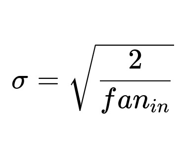
This is based on the idea that ReLU activations zero out about half the inputs, so we want a slightly larger variance for the weights to maintain signal flow. In practice, the weights can be sampled from either a normal or a uniform distribution, both scaled by this standard deviation factor.

Bias Initialization

Biases often default to zero initialization. The rationale is that having an excessively large or small bias at the start can shift the outputs too much. In practice, setting biases to small constants or zeros is standard and is usually sufficient for most networks.

Practical PyTorch Code Examples

It is straightforward to define a custom initialization function and apply it to your model. Below is a PyTorch snippet showing how you can manually initialize the parameters of a simple neural network:

import torch
import torch.nn as nn
import torch.nn.functional as F

class CustomNet(nn.Module):
    def __init__(self):
        super(CustomNet, self).__init__()
        self.fc1 = nn.Linear(128, 64)
        self.fc2 = nn.Linear(64, 10)

    def forward(self, x):
        x = F.relu(self.fc1(x))
        x = self.fc2(x)
        return x

def init_weights(m):
    if isinstance(m, nn.Linear):
        # Using Xavier Normal
        nn.init.xavier_normal_(m.weight)
        # Bias set to zeros
        nn.init.zeros_(m.bias)

model = CustomNet()
model.apply(init_weights)

In this example:

• We define a small network with two fully connected (Linear) layers.

• We create a helper function init_weights that uses isinstance checks on each layer to see if it is a nn.Linear.

• For each nn.Linear, we apply Xavier normal initialization to the weight tensor, and zero out the bias.

Other built-in initializers in torch.nn.init include:

• nn.init.xavier_uniform_

• nn.init.kaiming_normal_

• nn.init.kaiming_uniform_

• nn.init.zeros_

• nn.init.ones_

• nn.init.constant_

  Importance of Fan-in and Fan-out

  The parameters fan_in and fan_out define how many neurons connect into a layer and how many neurons this layer outputs to, respectively. These values are crucial for controlling the variance of the weights. The fundamental goal is to ensure that the signal (and gradient) does not diminish or explode as it passes through the network layers.

  Additional Notes

  While explicit initialization is useful, sometimes sticking with PyTorch’s default layer-wise initialization is sufficient for standard architectures. However, understanding and customizing initializations is essential when:

  • Dealing with novel architectures or activation functions.

  • Facing training instability and diagnosing gradient explosion or vanishing.

  • Reproducing research papers where specific initialization schemes are mandated.

  How to Manage Different Layer Types

  In larger architectures, you may have different types of layers (e.g., convolutional, linear, batch normalization). You can extend the same approach with PyTorch’s apply method but with more specialized checks, for example:

  def custom_init(m):
      if isinstance(m, nn.Conv2d):
          nn.init.kaiming_uniform_(m.weight, nonlinearity='relu')
          nn.init.zeros_(m.bias)
      elif isinstance(m, nn.Linear):
          nn.init.xavier_normal_(m.weight)
          nn.init.zeros_(m.bias)
  
  model.apply(custom_init)
  

  By customizing for each layer type, you can pick the initialization strategy best suited for that layer’s role and activation function.

Follow-up Questions

Why is Xavier Initialization Often Used for Tanh or Sigmoid Activations?

Xavier initialization balances the variance across layers. For activation functions like tanh or sigmoid that can saturate, keeping the outputs within an appropriate range helps avoid situations where gradients become extremely small (due to the flat regions of those activation curves). Without such balancing, the network can get stuck in near-saturated states.

What Happens If We Use Kaiming Initialization with Sigmoid or Tanh?

Kaiming initialization is designed primarily for ReLU-based activations, which have different variance considerations than sigmoid or tanh. Using Kaiming for sigmoid or tanh may work in some cases, but it can lead to suboptimal convergence. Since Kaiming initialization includes a factor of 2/fan_in tailored for ReLU’s zeroing effect, it may not perfectly match the behavior of saturating activations.

Why Do We Often Initialize Biases to Zero?

Bias terms control the baseline offset of the layer’s output. When using random initial values for biases, there is a risk of pushing outputs into nonlinear saturation too early or introducing an arbitrary offset that lengthens training time. Setting biases to zero or a small constant helps ensure that each neuron’s output starts with a relatively neutral offset, making training more stable in most scenarios.

How Do We Decide Between Using Normal or Uniform Distributions?

It often comes down to preference, empirical results, or guidelines in literature. Xavier and Kaiming initializations both come in normal and uniform variants. Usually, uniform initialization might keep values in a defined range, while normal initialization can have occasional outliers due to the tails of the distribution. In practice, both forms have been successful across different network configurations, and many modern papers or frameworks rely on normal initialization for convenience.

What if We Observe Vanishing or Exploding Gradients Despite Proper Initialization?

Initialization is only part of the equation. Other factors influencing gradient stability include:

• Depth of the network: very deep networks are prone to vanishing/exploding gradients.

• Choice of activation function: saturating activations exacerbate these problems.

• Improper learning rate: too large a learning rate can explode gradients, whereas too small can impede training.

• Batch normalization or residual connections: these are often introduced to tackle exactly these issues alongside careful initialization.

Sometimes, combining a good initialization scheme with normalization layers, skip connections, or well-tuned learning rates is required to eliminate vanishing or exploding gradients in deep architectures.

Below are additional follow-up questions

How does weight initialization differ for RNN-based architectures, and what are the potential pitfalls there?

When dealing with Recurrent Neural Networks (RNNs) or their variants like LSTM and GRU, initialization can be more complex compared to feed-forward networks. Unlike a simple Linear or Conv layer, recurrent layers maintain hidden states that influence future computations. Key points include:

• Multiple Weight Matrices: For LSTM cells, each gate (input, forget, output, and candidate cell gate) has its own parameter matrices. Default PyTorch initialization typically places certain sub-matrices in orthogonal or uniform distributions. However, customizing these initializations may be needed if your data or architecture is non-standard.

• Exploding or Vanishing Gradients: RNNs are more prone to these issues because of long sequences and repeated multiplication by weight matrices. An initialization that is slightly too large can accelerate exploding gradients, while too small can cause vanishing gradients quickly.

• Orthogonal Initialization: A common practice for the recurrent weight matrices in RNNs is to initialize them orthogonally. This helps preserve the gradient flow over multiple time steps. However, orthogonal initialization might need additional care if you use advanced gating mechanisms.

• Hidden-State Bias and Forget Gate Bias: For LSTMs, researchers often initialize the forget gate’s bias to a positive constant (for instance, 1.0) to encourage the model to “remember” more at the start of training. Using a zero bias in the forget gate can lead to underutilization of the cell’s memory capacity initially.

• Edge Case – Small Batch Sizes: When the batch size is tiny or if each sequence is short, random initialization might have a more pronounced effect on training. You might see large performance fluctuations. A more careful choice (e.g., a smaller variance) can help stabilize the updates in those scenarios.

How do initialization strategies change in Generative Adversarial Networks (GANs), and are there any special considerations?

GANs typically consist of a generator and a discriminator, each with different objectives. Subtle initialization details can affect the delicate balance of training. Key considerations:

• DCGAN Initialization Convention: A well-known approach is to initialize all convolutional and transposed convolutional layers in both generator and discriminator with a normal distribution having mean=0 and std=0.02. This was popularized by the authors of DCGAN (Deep Convolutional GANs). It keeps the initial scales of outputs in a range conducive to stable adversarial training.

• Balancing Generator and Discriminator: Since the generator tries to fool the discriminator while the discriminator tries to distinguish real from fake, an overly large or small initialization can cause one of them to dominate training early on. This imbalance might stall training or push it into mode collapse.

• Bias Terms in BatchNorm Layers: In some GANs, the effect of BatchNorm bias initialization is significant for the generator. If the bias is set incorrectly, the generator’s outputs might start in a degenerate region and fail to produce diverse samples.

• Edge Case – Different Architectures: Some advanced GAN variants (e.g., StyleGAN) use progressively growing networks or style-based generative layers with unique initialization methods. Replacing those with default or naive initializations could severely degrade performance or training stability.

If we are doing transfer learning or fine-tuning from pretrained weights, how does initialization come into play?

When starting from pretrained weights, your network already has a non-random initialization that captures useful representations from a large dataset such as ImageNet. Potential nuances include:

• Freezing vs. Partial Fine-tuning: If you freeze earlier layers, then initialization matters primarily for the newly added layers (e.g., a custom classifier). Those new layers typically get randomly initialized (say, Xavier or Kaiming), while the frozen layers retain the pretrained values.

• Non-i.i.d. Transfer: If your source domain differs substantially from the target domain, the pretrained weights might not serve as an optimal starting point. In that case, you might consider a more advanced scheme like layer-wise tuning or re-initializing certain blocks if they lead to negative transfer.

• Learning Rate Scheduling: Even with good initialization from pretrained weights, an improper learning rate can cause overfitting or underfitting. Many practitioners use smaller learning rates for pretrained layers and larger learning rates for newly initialized layers. This strategy ensures stability while still allowing the new layers to adapt sufficiently.

• Edge Case – Mismatch in Input Channels: Sometimes, the new task has a different number of input channels (e.g., from RGB to single-channel input). One workaround is to replicate or average the pretrained weights across channels. Another is to freeze part of them and randomly initialize the rest.

Can using inconsistent initialization schemes across different layers lead to issues, and how can we spot or mitigate them?

In large networks with diverse layer types, it’s possible that different initialization schemes (e.g., Kaiming for some layers, Xavier for others) might lead to mismatched scale distributions early in training. This causes:

• Discrepancies in Gradient Magnitudes: If the variance from one block is significantly larger, it can overshadow gradients coming from other blocks, leading to a skewed update distribution.

• Training Instability: Mixed distributions can escalate the risk that some layers explode while others remain near zero outputs, especially if the activations are sensitive to scale (e.g., ReLU vs. tanh).

• Debugging Strategy: Monitor gradient norms per layer. If you see one layer’s gradient norm is always orders of magnitude larger or smaller, it might be an indication that the initialization or learning rate for that layer is out of sync. Tools like TensorBoard histograms can help visualize weight distributions and check for anomalies.

• Mitigation: Choose a consistent or at least a well-justified scheme across layers that share similar activation functions. For example, if the entire network is ReLU-based, using Kaiming for all layers ensures a consistent scale. For layers with different activations, unify the approach by carefully selecting the initializer that best matches each activation’s theoretical requirements.

Is there a scenario where we need a custom or data-dependent initialization, and how would we implement it in PyTorch?

Yes, some specialized architectures or tasks call for data-dependent initialization. For instance, in certain flows-based models or normalizing flow architectures, the initial transformation layers might be computed in reference to actual data statistics. Key points:

• Data Statistics: Before training, you can run a forward pass over a sample of your dataset to capture means or variances. Then use those to determine the initial scaling of certain layers so that outputs align with a desired distribution.

• Implementation Steps:

  1. Build the model with placeholders for weights.

  2. Make a forward pass with a batch of real data.

  3. Calculate the required weight or bias values based on the statistics of intermediate outputs.

  4. Assign those values using with torch.no_grad(): m.weight.copy_(...).

• Pitfalls:

  • Overfitting to the Batch: If the batch used for initialization is not representative, you might get skewed parameter settings. Use a sufficiently large or diverse sample.

  • Compatibility with BN or LN: If your network also includes Batch Normalization or Layer Normalization, data-dependent initialization might interact with these layers. Carefully test if the combined effect is stable.

• Example Use Case – Variational Autoencoders: Some advanced VAEs or normalizing flows rely on approximate covariance matrices from the data to initialize certain transformation layers. A mismatch between the estimated distribution and actual data distribution can degrade performance if done incorrectly.

In extremely deep architectures (e.g., hundreds of layers), is initialization alone enough to address vanishing or exploding gradients?

No, once networks become very deep, even theoretically sound initialization might be insufficient. Key details:

• Residual and Skip Connections: Modern deep architectures like ResNets mitigate gradient problems by incorporating skip connections. This is not strictly about initialization but helps ensure that gradients have multiple, more direct pathways to flow backward.

• Normalization Layers: Techniques such as Batch Normalization, Layer Normalization, or Group Normalization can further stabilize gradients. They can also reduce the network’s sensitivity to certain initialization choices.

• Convergence Issues: In extremely deep models, a small deviation in initialization can accumulate across many layers. This can quickly blow up or diminish signals if unaddressed. Hence, it’s crucial to pair an appropriate initialization scheme with architectural design strategies like skip connections and normalization layers.

• Monitoring Tools: Checking gradient magnitudes at various depths of the network can reveal if vanishing or exploding is occurring. If issues persist, consider adjusting the initialization scale, employing advanced regularization methods, or reevaluating the architecture.

Do unusual activation functions (e.g., Swish, GELU, etc.) require unique initialization strategies?

Some modern activations do not precisely follow the assumptions of ReLU or tanh-based derivations (like the fan_in or fan_out approximations used in Kaiming or Xavier). Nonetheless, many still rely on Kaiming or a slight variant:

• Swish, GELU, and SELU: SELU has a specific initialization known as Lecun Normal, which sets the variance to 1/fan_in. With Swish or GELU, people often still default to Kaiming. Empirically, it tends to work adequately, although there may be room to fine-tune the variance hyperparameters if the network remains unstable.

• Data-Driven Tuning: In some research contexts, the approach is to start with Kaiming or Xavier, then do a grid search on the initialization gain factor to see if a small tweak helps. This is because the effective slope or shape of the activation can differ from ReLU or tanh.

• Edge Case – Custom Activation: If you invent or adopt a niche activation function, the established theoretical justifications for standard initializations may not hold. In these rare cases, analyzing the activation function’s approximate variance and gradient behavior might require deriving a custom scaling factor for your initialization.

Could dimension or shape mismatch in weights or biases cause silent issues during initialization?

Yes, dimension mismatches can sometimes get masked or lead to runtime errors that appear unrelated to initialization:

• Broadcasting Problems: If the shape used for bias initialization is incorrect, PyTorch might attempt broadcasting that leads to unexpected results. Generally, PyTorch will raise an error if the dimensions are incompatible, but subtle off-by-one dimension issues can result in an unintended distribution of parameter values.

• Layer Replacement or Resizing: During prototyping, you might replace a nn.Linear(in_features=128, out_features=64) with a different dimension but forget to update the custom initialization code that expects a 128×64 shape. This mismatch can lead to partial initialization or an exception. Always double-check the shape constraints.

• Debugging Strategy: Print out or log .shape for each parameter after applying model.apply(init_function). Confirm that each dimension matches your intended layer specification. If something is off, you’ll catch it early.