
ML Interview Q Series: How can we explain loan denials without directly examining the model’s feature weights in binary classification?

📚 Browse the full ML Interview series here.
Short Compact solution
One way is to rely on partial dependence plots (or response curves). These plots let us see how varying one feature at a time, while holding other features constant, affects the predicted probability of loan acceptance. We do not have to look at actual internal weights to get an idea of why the model might be rejecting an applicant. Instead, if one of the plots reveals that lower FICO scores, for instance, strongly correlate with rejection, we can point out that the applicant’s relatively low FICO score is likely influencing the negative decision.
Concretely, suppose four applicants share similar income, debt, and number of credit cards, but differ in FICO scores. If the two applicants with lower FICO scores are turned down while the other two are accepted, it strongly suggests that FICO score is what drove those denials. Thus, even without accessing the exact learned weights, we can infer that a low FICO score is the explanatory factor.
Comprehensive Explanation
Partial dependence plots are an intuitive technique to uncover how each individual feature influences the model’s outcome, one at a time. The main concept is that for a given feature, we vary its possible values over a range while keeping the other feature values constant, and then compute the average model output. This approach gives a high-level view of the model’s sensitivity to each feature, without revealing the exact internal coefficients or structure.
Because partial dependence plots typically represent an aggregated effect, they allow us to say something like, “For applicants whose FICO score is around 600, the model’s predicted loan approval probability is significantly lower than for those at 700 or above.” This can be used to generate a reason for a particular individual’s denial—namely, that their FICO score is well within the range where the partial dependence plot dips toward a negative outcome.
How Partial Dependence is Computed
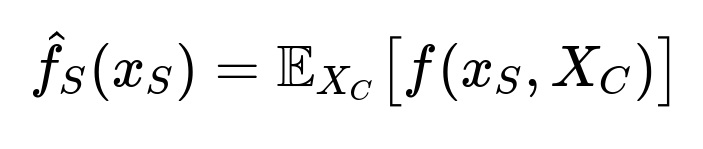
In simple terms, if the model’s prediction function is denoted by f(x), where xx is the set of input features, then the partial dependence function for a feature subset S can be thought of as:
Why This Approach Makes Sense for Loan Rejections
If an applicant is denied a loan, you can look at the partial dependence plots for each feature (for instance, FICO score, debt, annual income, number of credit cards). Whichever feature’s partial dependence curve shows a sharp decline around that applicant’s specific value is a likely candidate for explaining the model’s negative decision. This method neither requires revealing the proprietary details of the internal model nor analyzing raw feature importances. Instead, you only need to show how the predicted outcome changes as you vary the applicant’s feature value while other things stay equal.
Implementation in Practice
A practical approach might involve using frameworks such as scikit-learn’s PartialDependenceDisplay (for classical ML models) or other libraries that can produce partial dependence plots. Once you have fitted your model (whether it is a random forest, gradient boosting, or even a neural network that supports such interpretability tools), you generate these plots on the training set or a representative sample. Then, for any denied individual, you can:
Locate their position on each partial dependence curve.
Compare it to thresholds or turning points the curve displays.
Provide a data-driven statement: “According to our model’s learned patterns, people with a FICO score under 650 tend to have a significantly lower chance of acceptance.”
Potential Pitfalls
When features are highly correlated, partial dependence plots can become misleading because varying one feature independently while keeping others fixed may never occur in real data. Additionally, partial dependence is an “average” effect, so it does not always describe an individual case perfectly. For a single applicant’s explanation, local methods such as LIME or SHAP might offer additional clarity. However, partial dependence remains a strong option for a high-level, easy-to-implement approach that does not disclose proprietary model internals.
What if the model is extremely complex?
Partial dependence methods can be computed on most machine learning algorithms, including tree-based ensembles and neural networks. Complexity may increase the computation time, but the interpretability advantage often justifies the extra overhead. The user can further sample the dataset to make computations more tractable.
Follow-Up Questions
How do we handle feature correlation when using partial dependence?
Correlated features can cause partial dependence plots to be unrepresentative, because varying one correlated feature over a broad range may be inconsistent with the typical relationship of the other features. This might lead to unrealistic or non-occurring data points when creating the curve. A common workaround is to compute partial dependence only within a realistic domain. Another approach involves conditional dependence plots, where you condition on the distribution of correlated variables instead of treating them as completely independent. In practice, SHAP values or local methods can offer finer-grained interpretations that account for correlation by examining real data neighborhoods rather than artificially fixing certain features.
How can we explain individual instances if partial dependence is an average effect?
Partial dependence plots provide a holistic view of how a feature shifts predictions on average. For a specific applicant, we may need local interpretability methods. These techniques, such as LIME or SHAP, create perturbed samples around that single point and see how the model’s prediction changes, attributing local “importance” to each feature. Hence, to provide a more personalized justification, we would say, “Based on local analysis of your features, the main driver behind your rejection was your FICO score being in a critical range.” In other words, partial dependence gives a broad overview, while local methods tailor explanations to each individual.
What if partial dependence suggests a different reason than feature importances?
Feature importances are often aggregated measures (for instance, how much each feature reduces impurity in a tree-based ensemble). Partial dependence, on the other hand, focuses on how the predicted value changes when one feature shifts. It is entirely possible for a feature that is globally “less important” to have a high partial dependence effect at certain intervals of its range. This discrepancy can arise because feature importances might look at the entire data distribution, whereas partial dependence picks up on local or mid-range variations. The correct approach is to combine these metrics carefully and look at local explanations if you need clarity for a specific decision boundary.
Could we use alternative methods like SHAP or LIME?
Yes. SHAP and LIME are more localized approaches that attempt to explain individual predictions. SHAP in particular offers a theoretically grounded measure of feature contribution by connecting to Shapley values from cooperative game theory. If partial dependence plots are not sufficiently granular, or if we need a more rigorous local explanation, SHAP or LIME can tell us precisely how much each feature contributes to a single prediction. Yet partial dependence remains a simpler, more intuitive method for providing a broad, global picture of how the model responds to different values of a given feature.
How do we know if this approach is legally or ethically acceptable?
In many jurisdictions, lenders must provide understandable reasons for loan denials. Partial dependence or similar explanation methods can comply with these requirements by giving applicants plausible, data-based justifications (for example, insufficient FICO score, too high a debt-to-income ratio, etc.). However, legal frameworks like the Equal Credit Opportunity Act or other fair lending laws might also demand that your model does not discriminate based on protected classes. As such, you should combine interpretability with rigorous bias audits and fairness checks. If your method reveals consistent bias or unusual partial dependence for sensitive groups, you would need to address that prior to deployment.
Implementation Details in Python
Below is a sketch of how one might generate partial dependence plots using scikit-learn in Python. Assume we already have a dataset with features [“FICO_score”, “Debt”, “Income”, “NumCreditCards”], and a fitted gradient boosting model named gb_model.
import numpy as np
import matplotlib.pyplot as plt
from sklearn.inspection import partial_dependence, PartialDependenceDisplay

# Suppose X is your feature matrix, y is your labels
# and gb_model is a trained GradientBoostingClassifier

features_to_plot = [0, 1, 2, 3]  # Indices of features in the dataset

fig, ax = plt.subplots(figsize=(12, 8))
display = PartialDependenceDisplay.from_estimator(
    gb_model,
    X,
    features_to_plot,
    kind='average',
    ax=ax
)
plt.show()
This script generates partial dependence curves for each of the specified features. You could then observe how the model’s predicted probability of loan approval varies across different values for each feature. For a particular rejected applicant, you would pinpoint their feature values on these plots to see which curves correspond to a lower likelihood of acceptance.
By following this procedure, you derive an understandable, approximate explanation for why an individual might have been denied, all without opening up the black box of model internals or analyzing numeric weight values directly.
Below are additional follow-up questions
How do partial dependence plots handle out-of-distribution feature values?
Partial dependence plots (PDPs) typically assume that the range over which you vary a feature is relevant and representative of the original training data. However, if you push a feature far outside the domain in which the model was trained (e.g., a FICO score much higher or lower than anything in the training set), PDPs might display misleading or unreliable trends. Models extrapolate differently—some can gracefully handle it, others predict nonsensical results.
One practical pitfall arises if your training data’s FICO scores span, for instance, 400 to 850, but you draw a partial dependence plot that extends from 200 to 950. The model never saw data in that range, so the plot could be entirely hypothetical. This can be problematic in explanations for real users who might assume the model accurately handles that region.
To mitigate this, you can:
Restrict PDP generation to the actual min–max range of each feature in the training set, or to the most common feature intervals.
Annotate or highlight that beyond certain limits, the predicted behavior is an extrapolation that might be less reliable.
Are there scenarios where partial dependence plots are not feasible due to data size or computational constraints?
If you have a very large dataset with high-dimensional features, generating PDPs can become computationally expensive. This is especially true when you:
Have to iterate through all instances for the marginalization (or a large subset) to compute each point on the plot.
Use very complex models (e.g., large neural networks) that take longer to evaluate.
In practice, for massive datasets, you might:
Downsample the data to reduce computation time, hoping to preserve representative distributions.
Employ approximate methods (e.g., using a random subset of feature values for XC when calculating the expectation).
Leverage GPU acceleration if your model supports it.
You must ensure that the downsampled data still captures essential relationships or risk introducing biases or losing important information relevant to interpretability.
What if two features always appear together in reality (e.g., perfect or near-perfect correlation)?
PDPs vary a single feature (or a small subset) over a range while holding others constant. If you have two features that are always coupled—for example, “Income” and “Debt-to-Income ratio”—it may be impossible (or at least highly unrepresentative) to vary one without also changing the other. Consequently, the partial dependence curve might depict scenarios that never happen in the real world.
Such unrealistic scenarios can lead to poor or downright misleading interpretations. In these cases:
Conditional partial dependence plots, which fix the correlated features according to their joint distribution, might yield more realistic insights.
Techniques like SHAP or local methods can better handle correlated features by constructing local perturbations that respect the actual correlation structure in the data.
How do we handle scenarios where categorical variables have many levels or complex interactions?
For categorical variables with many distinct categories—such as region codes, job types, or product IDs—PDPs can get cluttered or lose interpretive power when plotted on the x-axis. If there are dozens or hundreds of categories, your partial dependence plot for that feature becomes difficult to read.
Moreover, interactions between categories and numeric features can create unique patterns that aren’t captured by looking at one feature’s PDP in isolation. For these situations:
Consider grouping categories by higher-level logic (e.g., “job sector” instead of specific job titles).
Use two-way partial dependence plots that attempt to show interactions between a categorical and a numeric feature, though this increases complexity.
If the number of categories is extremely high, techniques like embedding them (in deep models) or target encoding (in tree-based models) might complicate interpretability further, so local explanations (e.g., LIME, SHAP) can be more helpful for specific instances.
How do we interpret partial dependence if the model is extremely non-monotonic?
Some features could influence the outcome in a non-monotonic way—for example, a certain debt level might be okay, but too low or too high signals risk. The PDP might show peaks and dips. It can be confusing for users to interpret multiple local maxima or minima on the plot.
In those cases:
The explanation should highlight that the feature has a complex relationship with the outcome. For instance, very low debt might indicate insufficient credit history, while very high debt implies risk.
Combining PDP with additional visualizations—like ICE (Individual Conditional Expectation) plots, which display one line per instance—helps differentiate whether the non-monotonic pattern is a universal effect or something that affects only a few subgroups in the data.
Can partial dependence plots mislead us if the model has strong feature interactions?
If the model’s predictions depend heavily on interactions between features—say, debt only matters significantly when income is below a certain threshold—then a single-feature PDP might average over many different scenarios and fail to reveal that important conditional relationship. This can underrepresent how impactful the feature can be for certain slices of the data.
To address strong interactions:
Use two-way or multi-way PDPs, though these can get visually challenging. For instance, you can examine partial dependence over the grid of (Debt, Income).
Employ local explanation methods for each specific denied applicant to see how the interplay of Debt and Income individually shaped their prediction.
Understand that a standard PDP is a marginal effect, so if the model is deeply non-linear with multiple higher-order interactions, a single-feature PDP is only a broad stroke.
What happens if the partial dependence suggests multiple features might cause the rejection? How do we choose which reason to report?
In real-world loan decisions, applicants often fail on multiple criteria simultaneously. PDP might reveal that both low FICO score and a high number of credit cards (or high debt) drive the outcome down. Reporting every possible factor can overwhelm the applicant.
A balanced approach is:
List the top one or two factors that have the most significant partial dependence effect near the applicant’s feature values.
Clarify if there are secondary factors that also negatively contributed.
Provide actionable feedback: “Your FICO score and outstanding debt were the primary reasons. Improving your credit score or reducing debt may increase your chances of approval.”
How do we handle time-varying features or data drift when using partial dependence?
In some lending systems, features like employment length or credit utilization change over time. A PDP computed on historical data may not remain accurate if the distribution of features drifts significantly. For instance, after an economic shift, typical income or debt levels might change.
If the data is non-stationary:
Update or recalculate partial dependence plots periodically (e.g., monthly, quarterly) to ensure they reflect the current data distribution and model behavior.
Track concept drift indicators. If the model is retrained regularly, regenerate updated PDPs for interpretability in the new environment.
Warn that the partial dependence plots are valid for a certain timeframe and might need re-interpretation if macroeconomic conditions shift drastically.
How do we prevent gaming of the system if we publicly disclose partial dependence explanations?
Revealing that “a FICO score below 650 strongly reduces approval chances” may lead applicants to artificially inflate their FICO or attempt to manipulate other features the model depends on. This is an inherent risk when offering transparent explanations. If gaming is a concern:
Implement checks to detect suspicious or abrupt changes in features, such as verifying income or credit usage through external data sources.
Apply anti-fraud or consistency checks that go beyond the model’s raw features alone.
Maintain a balance between necessary transparency for legal or ethical reasons and protective measures against malicious exploitation.
How does partial dependence differ from counterfactual explanations?
Counterfactual explanations answer the question: “What minimal changes to the input features would have led to an approval instead of a rejection?” For instance, a counterfactual method might say, “If you had reduced your debt from $10,000 to $7,000, you would have been approved.” Partial dependence, by contrast, is more general, showing how predicted outcomes shift across the range of a feature in aggregate.
If you need actionable advice for a specific individual, counterfactuals could be more meaningful. PDP is more of a global interpretability tool that is not inherently personalized, though it can be used to glean which features matter. Combining partial dependence with counterfactual logic can yield both broad insight (“FICO score is crucial”) and specific advice (“Pay off at least $3,000 of your debt”).
What if partial dependence highlights potentially sensitive features (e.g., age or location)?
In many jurisdictions, using sensitive attributes like age or location explicitly in a loan approval model can trigger regulatory scrutiny. Even if such features are technically permitted, showing that partial dependence drastically shifts for certain demographic groups can lead to accusations of unfair lending.
If a PDP reveals a stark difference for a protected group, you should:
Check if this is a proxy for legitimate risk factors or an unintended bias in the data.
Consider removing or carefully regularizing that feature to mitigate disparate impact.
Perform fairness or disparate impact analyses to ensure the model complies with ethical and legal standards.