ML Interview Q Series: How can you define and compute the Frobenius norm of a matrix?

📚 Browse the full ML Interview series here.

Comprehensive Explanation

The Frobenius norm of a matrix is a specific way to measure the size (or magnitude) of that matrix, treating the matrix almost like a long vector of its entries. It is particularly useful in contexts such as low-rank approximations, regularization, and optimization problems in machine learning. One of its key properties is that it is unitarily invariant, meaning that certain transformations (like multiplication by orthogonal or unitary matrices) do not change its value.

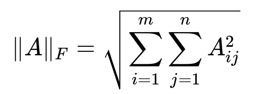
Where A is an m x n matrix, A_ij is the element in the i-th row and j-th column, m is the number of rows, and n is the number of columns. The core idea is to sum up all the squares of the individual entries and then take the square root. You can think of this as simply extending the idea of the vector Euclidean norm to matrices.

When you calculate the Frobenius norm, you are effectively collecting every element in the matrix into one combined measure of magnitude. Another way to express it (in a text-based inline manner) is sqrt(Tr(A^T A)), where Tr is the trace operator. This trace-based expression is often used because it is elegant and connects to other concepts such as singular values.

The Frobenius norm is also equal to the square root of the sum of the squares of all the singular values of A. If sigma1, sigma2, ..., sigmar are the singular values of A, then the Frobenius norm is sqrt(sigma1^2 + sigma2^2 + ... + sigmar^2). This is why it is sometimes referred to as the Hilbert-Schmidt norm or the Schatten 2-norm.

It is important for many practical machine learning methods. For example, in matrix factorization tasks (like low-rank approximations) or in certain forms of regularization, one might penalize the Frobenius norm of a parameter matrix. This helps to smooth or reduce the overall magnitude of the parameters in a controlled fashion.

How does the Frobenius norm differ from other matrix norms?

The Frobenius norm differs from other matrix norms in its definition and in the geometric property it captures. Unlike the operator norm (or spectral norm) which is the largest singular value, the Frobenius norm involves the sum of the squares of all singular values. This means it is more sensitive to all entries in the matrix, not just the largest mode of variation.

In some problems, the spectral norm might be more appropriate if you only care about the dominant direction of the matrix transformation (largest singular value). However, in cases where you want to capture the entire “spread” of values (or the overall energy in all directions), the Frobenius norm is often preferred.

Why might one choose the Frobenius norm for regularization?

In many machine learning models, regularizing a matrix parameter with the Frobenius norm penalizes all coefficients in that matrix evenly. This ensures that no single coefficient or subset of coefficients becomes excessively large. It is akin to the L2 norm for vectors but extended to matrices. As a result, you get a smooth penalty that shrinks all entries proportionally, often making the optimization problem more tractable (for instance, it remains differentiable everywhere).

On the other hand, if you want to promote sparsity or rank constraints, the Frobenius norm might not be the best choice. For instance, if rank minimization is needed, the nuclear norm (sum of singular values) is more common. If you want to enforce entry-wise sparsity, an L1-based approach on each entry might be more suitable.

How do numerical stability and computational complexity factor in?

Computing the Frobenius norm is straightforward and typically involves an element-wise operation to sum the squares of all the matrix entries. This is generally O(mn) in complexity for an m x n matrix. From a numerical perspective, summing squares of many elements can lead to floating-point rounding issues if your matrix is extremely large or has a wide range of values. Commonly, one mitigates this with stable summation algorithms (for instance, using pairwise summation or Kahan summation) to reduce floating-point error.

What are potential edge cases or pitfalls?

A key pitfall is the scale of the entries in your matrix. If your matrix contains extremely large values or if it is extremely big, summing the squares can lead to overflow or numerical instability. Proper data scaling or using data types with higher precision can be important. Another edge case is if the matrix has many zeros, in which case the Frobenius norm might not be the best measure if you want to leverage that sparsity for analysis. There, alternative norms or specialized methods might be more appropriate.

Follow-up Questions

How does one compute the gradient of the Frobenius norm with respect to the matrix?

To compute the gradient of the Frobenius norm of A with respect to A, you can use the fact that the Frobenius norm is sqrt( sum of A_ij^2 ). The gradient is proportional to A itself. In particular, if you define f(A) = 1/2 * FrobeniusNorm(A)^2 = 1/2 * sum of A_ij^2 (which is often used in optimization for convenience), then the gradient with respect to A is just A. This linearity makes it a very convenient choice in gradient-based methods.

Could you illustrate a small example to ensure understanding?

Imagine a 2 x 2 matrix:

[ 2   3 ]
[ 1   4 ]

The Frobenius norm would be sqrt(2^2 + 3^2 + 1^2 + 4^2). That is sqrt(4 + 9 + 1 + 16) = sqrt(30). This is a straightforward extension of the Euclidean norm in vector spaces.

In what contexts do we see the Frobenius norm used most frequently in Deep Learning?

In many neural network regularization contexts, such as weight decay (L2 regularization) for matrix parameters, the Frobenius norm appears when you flatten the matrix into a vector and apply the L2 norm. For instance, if you have a weight matrix W in a layer of size input_dim x output_dim, the standard weight decay penalty is essentially the Frobenius norm of W (or squared Frobenius norm). This helps control overfitting by penalizing the overall magnitude of the weight matrix.

It is also relevant when measuring reconstruction error in tasks like autoencoder training or other factorization problems, where the objective might be to minimize the Frobenius norm of (Data - Reconstruction).

How is the Frobenius norm connected to the singular value decomposition?

If you take the singular value decomposition of matrix A (i.e., A = U S V^T for some unitary or orthogonal matrices U, V, and diagonal singular value matrix S), then the Frobenius norm is the square root of the sum of squares of the singular values (the diagonal elements of S). This decomposition-based view provides a strong link between the Frobenius norm and the concept of total energy or total variance captured by all the singular values of A.

This property also helps in ranking the contribution of each singular value to the overall norm. The spectral norm (largest singular value) focuses on the maximum singular value, whereas the Frobenius norm emphasizes the collective sum of squares of all singular values.

Could there be any relationship between the Frobenius norm and eigenvalues for symmetric matrices?

If a matrix is symmetric and positive semi-definite, its eigenvalues coincide with its singular values. In such cases, you can interpret the Frobenius norm as the square root of the sum of squared eigenvalues. That can be useful in certain formulations where you need to connect the norm to principal component analysis or covariance matrices.

All of these insights reinforce why the Frobenius norm is a common choice in many numerical linear algebra tasks and why interviewers often ask about it to test a candidate’s depth of knowledge in matrix operations and norms.