
ML Interview Q Series: How can you generate a classification prediction using a Logistic Regression approach?


📚 Browse the full ML Interview series here.
Comprehensive Explanation
Logistic Regression provides a way to estimate the probability that a given input x belongs to a certain class (often called the "positive" class). The core idea is to take a linear combination of the input features and transform it through the logistic (sigmoid) function. This transformation outputs a value p ranging from 0 to 1, which is then interpreted as the probability of the class label being 1.
The probability for class 1 can be computed by applying the logistic function to the linear score. Below is the key formula in its standard form:
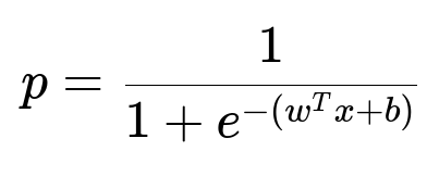
Here, w is the weight vector (one weight per input feature), x is the vector of input features, and b is a bias term (or intercept). The dot product w^T x is the weighted sum of the features, which is then shifted by b. The exponential function e^{-(w^T x + b)} compresses any real number into a positive scalar, ensuring that p is always between 0 and 1.
During the prediction phase, we often impose a threshold of 0.5. If p is at least 0.5, the predicted class is 1; if p is less than 0.5, the predicted class is 0 (though this threshold can be adjusted for different precision-recall trade-offs).
In practical settings, once you have trained a Logistic Regression model (i.e., fitted w and b by minimizing the loss function on the training data), you predict on a new sample x by simply computing the dot product plus bias, applying the sigmoid function, and then thresholding that probability.
Below is a brief Python code snippet using scikit-learn that demonstrates how to train and then predict with a Logistic Regression model:
from sklearn.linear_model import LogisticRegression
from sklearn.model_selection import train_test_split
from sklearn.datasets import make_classification
import numpy as np

# Generate synthetic binary classification data
X, y = make_classification(n_samples=1000, n_features=5, random_state=42)

# Split into training and test sets
X_train, X_test, y_train, y_test = train_test_split(X, y, test_size=0.2, random_state=42)

# Create and train the Logistic Regression model
log_reg = LogisticRegression()
log_reg.fit(X_train, y_train)

# Make predictions as probabilities
probabilities = log_reg.predict_proba(X_test)[:, 1]

# Convert probabilities to binary predictions using 0.5 threshold
predictions = (probabilities >= 0.5).astype(int)

print("Predicted probabilities:", probabilities[:5])
print("Binary predictions:", predictions[:5])
The above code shows the typical pattern of generating probabilities for each test instance and then converting those probabilities to binary labels with a 0.5 threshold.
What does the sigmoid function accomplish?
The sigmoid (or logistic) function transforms any real-valued number into the interval (0, 1). By mapping linear outputs to probabilities, the model can output how likely it is that the given input belongs to class 1. This probabilistic interpretation also lets you modify the threshold for different performance metrics such as recall, precision, or the ROC AUC score.
Why do we use the log loss as the objective function?
Logistic Regression is commonly trained by maximizing the likelihood of the data under the Bernoulli distribution assumption, which is equivalent to minimizing the negative log-likelihood (also called log loss). The log loss grows large if the predicted probability diverges significantly from the actual label, so minimizing it effectively aligns predicted probabilities closer to the true labels. This loss function is smooth and convex, making it tractable to optimize with gradient-based methods.
How can we interpret the model parameters?
Logistic Regression coefficients can be interpreted in terms of their effect on the log-odds of the outcome. When a coefficient w_j is positive, increasing the corresponding feature x_j increases the log-odds of predicting class 1. A negative coefficient implies that increasing x_j reduces those log-odds. The bias term b captures the base rate of the positive class in the absence of any predictive features.
What about decision thresholds other than 0.5?
Adjusting the threshold is common in imbalanced or specific business-critical applications. For example, if you want to minimize false negatives in a disease detection model, you might set a threshold below 0.5 so that you detect more positive cases (albeit at the expense of potentially more false positives). Such adjustments often come from analyzing the precision-recall trade-off or from cost-sensitive considerations.
How does regularization prevent overfitting in Logistic Regression?
In many implementations (e.g., scikit-learn), you can add an L2 penalty (or L1 in some cases) to the coefficients while training. This penalty term constrains the magnitude of the coefficients to avoid overfitting, where the model starts to memorize noise in the training data. The regularization strength is typically controlled by a hyperparameter (e.g., C in scikit-learn).
How do you handle imbalanced datasets?
When facing a dataset where one class is much rarer than the other, the model might learn biased probabilities. Strategies to deal with imbalance include:
Resampling techniques such as oversampling the minority class or undersampling the majority class.
Generating synthetic samples (SMOTE).
Adjusting class weights so that errors on the minority class are penalized more heavily.
Shifting the decision threshold to place more emphasis on the minority class.
Why might you choose Logistic Regression over more complex models?
Logistic Regression has the advantages of simplicity, interpretability, and fast training. It also performs well even with relatively small datasets, especially when the classes are linearly separable or nearly so. For high-dimensional settings, it is efficient and less prone to overfitting if proper regularization is applied. You can also gain insights into how each feature influences the outcome, which is harder with more complex models like random forests or deep neural networks.