
ML Interview Q Series: How can you carry out a time-series clustering approach that focuses on individual observations?


📚 Browse the full ML Interview series here.
Comprehensive Explanation
A common approach for clustering time-series data at the level of individual observations involves treating each separate time series as a distinct entity and measuring the similarity or distance between them. By doing so, we can form clusters of series that share common temporal behaviors. This process generally includes data pre-processing, selection of an appropriate distance metric, choice of clustering algorithm, and evaluation of results. Below is a detailed breakdown:
Data Pre-processing and Normalization
Time-series often come with inconsistencies such as differing lengths, missing values, or anomalies. The first step is to address these issues so that you can compare the time series in a fair and consistent manner. Typical steps involve:
Interpolating or imputing missing data.
Checking for outliers that could skew distance calculations.
Ensuring all series are of the same or comparable length, or applying time-warping methods if lengths differ significantly.
Normalizing the data so that larger scale series do not dominate smaller scale ones.
Choosing a Similarity or Distance Measure
Once the data is consistent, you need a way to measure how close or far apart any two time-series are. Euclidean distance, correlation-based measures, or more sophisticated methods such as Dynamic Time Warping (DTW) are commonly used. DTW is helpful if the series might be out of phase (shifted in time), but Euclidean distance is simpler and often works if series are well-aligned and share similar length.
Below is the Euclidean distance formula for two time-series X and Y, each of length T.
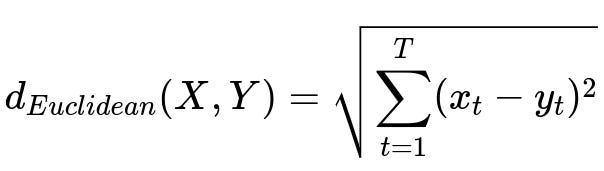
Where X = (x_1, x_2, ..., x_T) and Y = (y_1, y_2, ..., y_T) are two time-series, and T represents the number of time points in each series.
For time-series with shifts in timing or variable speeds, DTW helps align points in time to minimize the overall distance. DTW can handle stretching and compressing in the temporal dimension, but it comes with a higher computational cost.
Choosing a Clustering Algorithm
After deciding on the distance measure, common clustering algorithms include:
K-means: Typically requires using Euclidean distance and assumes each cluster can be well represented by a centroid. However, it does not directly handle non-Euclidean metrics like DTW unless modified with more advanced methods (such as k-medoids).
Hierarchical Clustering: Works with any distance measure and yields a dendrogram that you can cut at various levels to create different numbers of clusters. This method is often preferred when you do not know the number of clusters beforehand.
Density-Based Clustering: Algorithms such as DBSCAN may be used if clusters come in arbitrary shapes or you want to isolate outliers as their own clusters.
Assessing Cluster Validity
Evaluating clusters is often trickier with time-series data. You might:
Use internal metrics such as the Silhouette Coefficient, Calinski-Harabasz Index, or Davies-Bouldin Index to measure compactness and separation.
Evaluate domain-specific metrics, for instance, comparing cluster shapes to known patterns or checking if each cluster’s series make sense in the real-world context.
Perform external validation if you have labeled time-series.
Practical Implementation Example (Python with Euclidean Distance)
import numpy as np
from scipy.cluster.hierarchy import linkage, fcluster
from scipy.spatial.distance import pdist
import matplotlib.pyplot as plt

# Suppose data is a 2D numpy array of shape (num_series, series_length)
# data[i] represents the i-th time-series

# Step 1: Compute the distance matrix among all time-series
distance_matrix = pdist(data, metric='euclidean')

# Step 2: Perform hierarchical clustering
Z = linkage(distance_matrix, method='ward')

# Step 3: Choose number of clusters
clusters = fcluster(Z, t=5, criterion='maxclust')

# 'clusters' now holds the cluster label for each time-series
# You can visualize the dendrogram if needed:

import scipy.cluster.hierarchy as sch
plt.figure()
dn = sch.dendrogram(Z)
plt.show()
In a real scenario, additional steps such as missing data imputation, normalization, or specialized distance metrics like DTW would be integrated before or during the clustering phase.
Potential Follow-Up Questions
How do you address the issue of different time-series lengths when using Euclidean distance?
When time-series differ in length, direct Euclidean distance can be misleading. One solution is to truncate or pad the shorter series so that all series have the same length, but this might lose or distort information. Alternatively, methods like DTW handle differences in length and temporal alignment more flexibly by finding an optimal match between points of the two series. In practice, you would also consider how stretching or compressing segments impacts interpretability. If many time-series differ drastically in length, a more robust approach is to resample them to a common sampling rate or anchor them based on key events if domain knowledge allows.
Why might K-means not be ideal for time-series data with dynamic time-warping?
K-means relies on computing means of points to form centroids, which works best with Euclidean geometry. DTW defines distances in a manner that does not map naturally to a simple average. An alternative is to use k-medoids, also known as Partitioning Around Medoids (PAM), which selects actual data points as cluster centers. This avoids the need to compute an undefined mean of time-series under the DTW metric. Another consideration is the higher computational overhead when repeatedly calculating DTW distances within iterative processes.
How do you choose between hierarchical clustering, k-means, or density-based methods for time-series clustering?
In many real-world cases, hierarchical clustering is preferred when there is no clear guess about the number of clusters, and you want a dendrogram that can be cut at various levels. K-means (or k-medoids with an appropriate distance metric) might be used when you suspect the data can be reasonably captured with a fixed number of clusters, and you want a simpler interpretation of cluster centroids or medoids. Density-based methods like DBSCAN suit situations where you suspect clusters of arbitrary shapes or outliers. You might try several methods and compare their cluster validity measures or consult domain knowledge to decide which approach best captures the underlying structure.
What pre-processing strategies can handle noise in time-series before clustering?
Noise can be mitigated through smoothing methods like moving averages, Gaussian filters, or wavelet-based denoising. This ensures that small fluctuations do not dominate the distance calculation or clustering structure. If the noise is periodic or known to arise from sensor artifacts, domain-specific filtering methods can help isolate genuine signals from measurement errors. It is also important to consider the trade-off between removing noise and preserving essential patterns in the data.
How do you interpret and validate the resulting clusters?
Interpretation typically involves visual inspection of exemplar series from each cluster, looking for characteristic shapes or alignments that might correspond to meaningful patterns. You might compare the distribution of domain variables (like external labels or metadata) across clusters. If labeled data is partially available, external metrics like adjusted Rand index or normalized mutual information can provide a quantitative measure of cluster quality. Qualitative analysis with subject-matter experts is also common, particularly for time-series that arise in specialized fields (finance, healthcare, IoT, etc.).
How might you scale this approach to very large datasets?
Scalability becomes an issue because distance calculations can grow quadratically with the number of series. Options include:
Sampling or segmenting the dataset to reduce computation.
Using approximate algorithms for DTW or specialized data structures for fast nearest-neighbor searches.
Employing dimensionality reduction techniques such as PCA or autoencoder-based methods to represent each time-series with a compact feature vector, then performing clustering in the reduced space.
These strategies allow you to cluster time-series data that might otherwise be too large to handle with naive pairwise distances.