
ML Interview Q Series: How do clustering methods operate when tasked with anomaly detection, and what are their principal traits for identifying unusual data points?


Comprehensive Explanation
Clustering algorithms often serve as a foundation for anomaly (or outlier) detection. The central idea is to group data based on similarity and then identify observations that do not fall neatly into any cluster or lie too far from their assigned clusters. Below are key points about how clustering algorithms behave in the context of anomaly detection.
Concept of Cluster-Based Anomaly Detection
A straightforward strategy is to apply a clustering algorithm such as K-means, Gaussian Mixture Models, or DBSCAN to partition data into clusters. After creating clusters, each data point’s anomaly score can be measured by its distance to the cluster it belongs to. If that score crosses a threshold, the data point may be deemed anomalous.
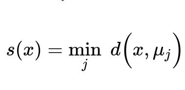
Where s(x) represents the anomaly score of data point x. The term d(x, mu_j) stands for the distance (often Euclidean in simple cases) between x and cluster center mu_j, and the function min_j ensures we consider the closest cluster. Points with large s(x) values (i.e., far from all cluster centers) can be labeled as anomalies.
All parameters in the formula are:
x is the data point for which we want an anomaly score.
mu_j is the center (or representative) of the j-th cluster.
d(x, mu_j) is the distance measure between x and the j-th cluster center. This could be Euclidean distance, Manhattan distance, or another metric chosen based on data characteristics.
Intuitive Explanation of Clustering Characteristics for Anomaly Detection
Clustering algorithms bring certain characteristics that can be advantageous or limiting for detecting outliers:
Local Density or Distance-Based Judgments Algorithms like DBSCAN consider the local density of points; regions with low density may indicate outliers. Others, like K-means, rely on distance to cluster centroids, marking any point lying far away from cluster centers as anomalous.
Sensitivity to Distance Metrics The concept of “far” or “close” is wholly dependent on the distance metric chosen. In high-dimensional settings, Euclidean distance can become less reliable due to the curse of dimensionality, making it challenging to separate normal points from outliers effectively.
Choice of Cluster Number For algorithms like K-means, you need to define the number of clusters (K). If K is not chosen thoughtfully, the boundary between “normal” clusters and anomalies might be poorly defined. Approaches like DBSCAN try to bypass this by discovering the number of clusters from data; however, DBSCAN also requires parameters like epsilon and min_samples, which strongly affect outlier detection performance.
Efficiency in Large Datasets Some clustering algorithms are computationally heavy in large-scale scenarios. K-means is relatively efficient, but DBSCAN and hierarchical clustering can struggle with huge datasets, thus possibly missing outliers or requiring approximate methods.
Robustness to Different Shapes Techniques like K-means typically discover spherical-shaped clusters. Data distributions that are elongated or manifold-like may not be well-captured, and anomalies in those structures might not be highlighted properly. By contrast, density-based methods can handle more complex cluster shapes.
Follow-Up Questions
How do you deal with the curse of dimensionality for cluster-based anomaly detection?
High-dimensional data often renders distance metrics less discriminative. One technique is dimensionality reduction, such as using PCA or t-SNE, to capture the essential structure in a reduced space. You can then apply clustering algorithms in this transformed lower-dimensional space, where distances become more meaningful for outlier detection. Additionally, methods like autoencoders can learn compact representations of high-dimensional data, making clustering and subsequent anomaly detection more effective.
What if you do not know the appropriate number of clusters beforehand?
Choosing the correct number of clusters remains a crucial problem. If you suspect a certain structure but cannot guess the number of clusters, you may use methods that infer the number of clusters automatically, such as DBSCAN or hierarchical clustering. Alternatively, you can use metrics like the silhouette score or the elbow method to get a rough sense of an optimal cluster count. In the context of anomaly detection, you can also examine how changing K affects the distribution of anomaly scores and pick a value that best separates normal points from potential outliers.
How do you handle scenarios where normal data and anomalies overlap partially?
Sometimes anomalies might overlap significantly with normal clusters, making it unclear whether a point is truly anomalous. This overlapping scenario can occur if there are multiple types of anomalies or if anomalies come from a distribution that partially resembles normal data. In practice:
You might combine clustering-based methods with supervised or semi-supervised approaches that incorporate labeled anomalies (if available).
You could adopt a probabilistic clustering approach, such as Gaussian Mixture Models, to get a probability distribution for each cluster. If a point has very low probability under all clusters, it can be flagged as an outlier.
Can you provide a Python snippet to illustrate cluster-based anomaly detection?
Below is a minimal example using scikit-learn’s K-means for clustering and labeling outliers if their distance from the nearest centroid exceeds a threshold:
import numpy as np
from sklearn.cluster import KMeans

# Synthetic dataset
np.random.seed(42)
normal_data = np.random.randn(200, 2)
outliers = np.random.uniform(low=-10, high=10, size=(10, 2))
data = np.concatenate([normal_data, outliers], axis=0)

# Fit KMeans
kmeans = KMeans(n_clusters=3, random_state=42)
kmeans.fit(data)

# Compute distance to closest cluster center
cluster_centers = kmeans.cluster_centers_
labels = kmeans.predict(data)

distances = []
for i, point in enumerate(data):
    center = cluster_centers[labels[i]]
    dist = np.linalg.norm(point - center)
    distances.append(dist)

distances = np.array(distances)

# Let's define an anomaly threshold (simplistic approach)
threshold = np.percentile(distances, 95)  # mark top 5% as outliers
anomaly_labels = distances > threshold

print("Number of anomalies detected:", np.sum(anomaly_labels))
In this snippet:
K-means is trained with 3 clusters on synthetic normal data plus a small set of outliers.
Each point’s distance to its assigned cluster center is measured.
Any point whose distance is above the 95th percentile is tentatively labeled as an anomaly.
You can refine the thresholding strategy or apply more advanced methods (like analyzing distance distribution) to determine outliers more precisely.
How do cluster-based methods compare with other anomaly detection approaches?
Other anomaly detection paradigms include:
Isolation Forest: Builds an ensemble of trees that isolate points. Those that get isolated quickly are considered anomalies.
One-Class SVM: Learns a decision boundary around normal data.
Statistical/Parametric: Assumes a distribution (for example, Gaussian). Points with low probability density under this distribution are treated as outliers.
Cluster-based methods can be intuitive and relatively straightforward to implement, but they may require proper tuning (cluster number or parameters like epsilon for DBSCAN) and can struggle in very high dimensions or complicated data distributions. On the other hand, specialized methods like Isolation Forest are specifically built for outlier detection and may handle complex data distributions more effectively with less parameter tuning.
How would you refine cluster-based anomaly detection in a real-world system?
In a practical production environment, you might:
Test multiple distance metrics (e.g., Euclidean, Manhattan) to see which best identifies known anomalies.
Investigate different clustering algorithms or combine them in an ensemble to get more robust outlier judgments.
Integrate domain knowledge to set or adapt thresholds dynamically. For example, if certain clusters inherently have greater variance, you might calibrate the anomaly threshold based on that cluster’s intrinsic spread.
Continuously monitor the results, collecting feedback on flagged anomalies from domain experts, and retrain or adjust parameters to reduce false positives and false negatives.
By iteratively refining these aspects, you can ensure that cluster-based anomaly detection remains accurate, reliable, and aligned with your application’s needs.
Below are additional follow-up questions
How do you select an appropriate distance metric for cluster-based anomaly detection?
Choosing the right distance metric is crucial because “distance” fundamentally drives how clusters form and subsequently how outliers are identified. While Euclidean distance is common, especially in lower-dimensional spaces, alternative metrics such as Manhattan distance, Chebyshev distance, or even more specialized metrics (e.g., cosine similarity in text/vector embeddings) may better reflect the nature of your data. If the data is high-dimensional or sparse (as is often the case in text data or some recommender systems), Euclidean distance might lose discriminative power due to the curse of dimensionality, so you might opt for more robust metrics that align with domain knowledge.
Potential pitfalls and edge cases
Using Euclidean distance in extremely high-dimensional data can result in nearly uniform distances, making it hard to separate normal from anomalous points.
Mixed-type data (e.g., categorical + continuous features) may need specialized distance functions (such as Gower distance).
In image embeddings, cosine distance might be more meaningful than Euclidean if vectors are normalized, because it emphasizes directional similarity over magnitude.
How do you approach clustering-based anomaly detection in a streaming or real-time environment?
In a streaming setting, data arrives continuously, and you need to detect anomalies on the fly. A naive approach of recalculating clusters from scratch on each new batch is typically impractical due to time constraints. Incremental or online clustering algorithms, such as online K-means or streaming variants of DBSCAN, can update cluster centers (or density estimates) as new data arrives without fully retraining from the beginning.
You might keep a rolling window of data, discarding the oldest points as new points come in, to ensure you detect anomalies under current conditions. The scoring of new points as outliers can be done by checking distances to existing cluster centers or local density thresholds.
Potential pitfalls and edge cases
Concept drift: The data distribution may shift over time, invalidating previously learned clusters. You need a strategy (e.g., gradually forgetting older data) to adapt to new patterns.
Resource constraints: Real-time systems often have strict memory and CPU limitations, so full-blown clustering on each incoming data point can be too expensive.
Delayed labeling: If you need human feedback to confirm anomalies, you might only get labels with some delay, complicating how quickly you can update your model.
How do you manage concept drift when using clustering methods for anomaly detection over time?
Concept drift refers to changes in data distribution over time, causing older clusters to become less representative of new data. In many real-world applications (e.g., monitoring network traffic, financial transactions), patterns evolve, and what was considered “normal” may shift.
A common approach is to apply a sliding or fading window: older data points or clusters gradually lose weight or are removed entirely. For example, if you maintain a set of cluster centers from the last N time steps, you can re-initialize, remove, or update clusters that no longer reflect current data. Some algorithms specifically track evolving clusters, merging or splitting them to handle drift.
Potential pitfalls and edge cases
Sudden or abrupt drifts: In cases like a major system upgrade or a global event, the data distribution might change radically, requiring re-initialization of clusters.
Slowly evolving distributions: Gradual drift might go undetected if the update mechanism is too rigid.
False anomalies: Genuine changes in user behavior or system behavior can look like anomalies if you do not adapt in time.
How do you add explainability to cluster-based anomaly detection?
While clustering can identify which data points deviate from typical cluster structure, offering explanations can be challenging. One practical approach is to examine how a data point differs from its cluster neighbors in specific features. You could look at feature-wise deviations: for example, compute the difference in each feature’s value between the outlier and the cluster centroid or median.
If you use tree-based methods or an ensemble approach along with clustering, you can leverage model interpretability methods like SHAP or feature importance measures to provide insights into which features contributed the most to a point being flagged as outlier.
Potential pitfalls and edge cases
High-dimensional data: Providing interpretability becomes more complicated as there are too many features for direct inspection. Feature engineering or dimensionality reduction can help.
Complex cluster boundaries: In non-spherical clusters (or those discovered by density-based methods), a simple distance to centroid explanation may be misleading. You might need to refer to local density profiles or nearest neighbor analysis.
User-level interpretability: If stakeholders are non-technical, it may be important to present explanations in intuitive, domain-specific terms.
How can we handle multi-modal or heterogeneous data in cluster-based anomaly detection?
Multi-modal data can include text, images, tabular features, or time series. A single clustering technique and distance metric might not be equally effective across all modalities. One approach is to create modality-specific embeddings or features (e.g., CNN-based embeddings for images, TF-IDF or transformer embeddings for text) and then combine them in a joint feature space.
You can apply dimensionality reduction or feature fusion strategies that transform diverse embeddings into a common representation. Once you have a consistent embedding, you can run clustering-based methods for anomaly detection. However, it’s essential to ensure that the combined feature space properly balances the contributions of different modalities (e.g., normalizing each embedding before concatenation).
Potential pitfalls and edge cases
Data alignment: For instance, if images and text must be matched (like product descriptions and product images), misalignment can create artificial anomalies.
Over-representation of dominant modality: If one modality is much richer than others, it can overshadow the contributions of the remaining modalities.
Computation cost: Processing and embedding multiple data types might be resource-intensive.
How do you handle extremely large datasets in a clustering-based anomaly detection workflow?
When data is very large, classical clustering algorithms like hierarchical clustering can become infeasible due to their high complexity. Even K-means can be expensive if the dataset is in the range of hundreds of millions of points. You can use approximate methods, mini-batch clustering, or sampling strategies.
For instance, you could perform mini-batch K-means, which updates cluster centers using small random batches, making it more scalable in memory and compute time. You can also do a two-phase approach: cluster a representative sample of the data and then map the remaining points to the nearest cluster centers, labeling outliers based on distance thresholds.
Potential pitfalls and edge cases
Sampling bias: If your sample does not properly represent minority classes or tails of the distribution, you might miss vital anomalous patterns.
Approximate results: Faster, scalable methods often introduce approximation. Verify that any approximation error does not mask anomalies.
Infrastructure limits: Even streaming or batch approaches require careful resource management (e.g., distributed computing solutions like Spark for large-scale clustering).
How do you detect anomalies when the data distribution is highly imbalanced?
In many real-world scenarios, anomalies are extremely rare compared to normal events (for example, fraud detection). A clustering approach might form clusters dominated by normal points and potentially ignore the minority distribution. One trick is to oversample or apply weighting methods that make rare patterns more visible to the clustering algorithm.
You can also do sub-clustering of minority data to identify internal structure within rare observations, which might clarify which minority patterns are actually normal in their own group and which are genuinely anomalous. This is somewhat akin to building separate clusters or density models for each class if you have partial labels.
Potential pitfalls and edge cases
Overfitting with oversampling: Artificially replicating rare data points can distort cluster boundaries.
Hidden sub-populations: If anomalies themselves have multiple modes (e.g., multiple types of fraud), a single cluster-based approach might lump them together or fail to detect smaller sub-groups.
Threshold choice: In an imbalanced scenario, even a small false-positive rate can generate a large volume of false alerts, so you need a strategy to calibrate threshold carefully.
How do you integrate partial labels for anomalies into a clustering-based approach?
Sometimes you have limited labeled anomalies from historical data or manual inspections. You can leverage these labels in a semi-supervised or weakly supervised learning setup. One method is to use a regular clustering pipeline but enforce constraints: labeled anomalies might be forced into their own clusters (or heavily weighted) so that the model isolates them from normal points more effectively.
You can also use a hybrid approach:
Train a supervised classifier on the small labeled anomalies plus normal data.
Use the classifier’s confidence scores to guide or initialize the clustering.
Refine the clusters to capture normal substructures while marking points with low classifier confidence as potential outliers.
Potential pitfalls and edge cases
Limited coverage: Labeled anomalies might not represent all possible anomalous patterns, leading to tunnel vision where new anomaly types are missed.
Noisy labels: If the few anomaly labels you do have are imperfect, they can mislead the clustering process.
Uncertain boundaries: Even with labels, anomalies might overlap with normal data, causing confusion in boundary assignment.
How would you adapt cluster-based anomaly detection for time-series data?
In time-series scenarios, the temporal context matters significantly. A point that is out of place in one time frame might be typical in another. You could extract temporal windows or sequence embeddings and then cluster these windows rather than individual points. When a new window does not match any existing cluster, you flag it as an anomaly.
Alternatively, you might combine time-series forecasting models (e.g., an LSTM that predicts future values) with a clustering approach on the forecast errors. If certain intervals exhibit unusually high reconstruction or prediction errors, they may indicate anomalies.
Potential pitfalls and edge cases
Lag dependencies: Simple clustering on raw time slices might miss important temporal correlations, e.g., daily or weekly seasonality.
Evolving patterns: Changes in seasonality or trends can cause normal behavior to appear as anomalies if the model isn’t updated.
High dimensionality: Each time window can be high-dimensional (especially if you track multiple variables), compounding the challenges of using distance metrics effectively.
How do you handle data drift that specifically affects the clustering boundary used for anomaly detection?
Even after forming clusters, small but incremental shifts in the data can gradually alter where the normal region ends and where anomalies begin. In practice, you can periodically re-estimate cluster boundaries or recalculate thresholds for anomaly scoring. For example, if using a distance threshold from cluster centroids to define outliers, you can dynamically adjust this threshold based on recent data distributions (e.g., a rolling quantile of distances).
In cases where the shift is more pronounced, you might need a heavier re-training step. Some practical strategies include:
Incremental or online updates to cluster parameters.
A re-initialization approach if you detect a major shift (e.g., by monitoring a drift detection metric).
Hybrid solutions that combine short-term online updates with less frequent “full” re-clustering.
Potential pitfalls and edge cases
Over-adaptation: If the system quickly adapts to new data, it might assimilate truly anomalous patterns into the “normal” region.
Delayed reaction: If updates are too infrequent, the system might continue to flag normal data (under the new distribution) as anomalous.
Balancing overhead and responsiveness: More frequent updates consume more computational resources, but less frequent updates can cause higher false positives/negatives.