ML Interview Q Series: How do Generative Adversarial Networks differ from autoencoders, and what sets them apart in how they learn latent representations and generate data?

📚 Browse the full ML Interview series here.

Comprehensive Explanation

Autoencoders and Generative Adversarial Networks (GANs) both belong to the family of neural networks that can learn representations of data in an unsupervised or semi-supervised manner. However, their goals and underlying training procedures differ significantly, leading to distinct usage scenarios and outcomes.

Autoencoders

An autoencoder is a neural network designed to learn a compressed, latent representation of input data by training the network to reconstruct the original input from this compressed encoding. The overall structure generally includes two main components:

• Encoder: Maps the input x to a latent representation z. • Decoder: Reconstructs the original data from the latent representation z.

The objective of an autoencoder is typically to minimize a reconstruction loss between the input x and the reconstructed output Dec(Enc(x)). For example, with a mean-squared error (MSE) reconstruction loss, the overall objective can be expressed as:

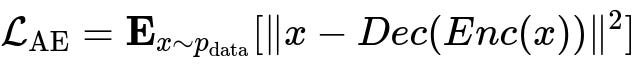
Here, x is a sample from the real data distribution p_data, Enc represents the encoder network, Dec is the decoder network, and the norm (‖ ‖^2) is the squared Euclidean distance (MSE) between the input x and its reconstruction Dec(Enc(x)).

Minimizing this reconstruction loss encourages the autoencoder to learn a latent code z that preserves essential information necessary for reconstructing x. Autoencoders are often used for tasks such as dimensionality reduction, denoising, anomaly detection, and feature learning.

Generative Adversarial Networks (GANs)

GANs consist of two networks that compete against each other in a minimax game:

• Generator (G): Takes as input a random noise vector z, sampled from some noise distribution (e.g., Gaussian), and outputs synthetic data G(z). • Discriminator (D): Takes an input (either a real sample from the dataset or a synthetic sample from G) and outputs a scalar representing the probability that the input is real.

GANs are trained by playing a minimax game between G and D. The discriminator tries to maximize its ability to distinguish real data from synthetic data, while the generator tries to fool the discriminator by generating samples indistinguishable from the real data. The canonical objective can be written as:

Here, x is sampled from the real data distribution p_data, z is sampled from the noise distribution p_z, D(x) is the discriminator’s estimate of the probability that x is real, and D(G(z)) is the discriminator’s probability that the generated data is real. The generator seeks to minimize this objective (fooling the discriminator), while the discriminator seeks to maximize it (correctly telling real from fake).

Because of this competitive, adversarial training, GANs produce highly realistic samples in many domains, such as image synthesis, style transfer, and text generation. However, they are more prone to training instabilities (e.g., mode collapse, vanishing or exploding gradients) and require carefully tuned hyperparameters and architectures.

Key Differences

• Data Generation vs. Reconstruction Focus. An autoencoder’s primary goal is to reconstruct its input using a latent space, while a GAN’s main goal is to generate new data that looks as real as possible to a discriminator.

• Training Objective. Autoencoders minimize reconstruction loss. GANs use an adversarial loss derived from a minimax game between two networks.

• Realistic Synthesis. GANs can generate extremely realistic samples after training, whereas standard autoencoders do not focus on generating new samples that look real; they simply reconstruct input data. Variants like Variational Autoencoders (VAEs) do focus on generative capability, but still differ from GANs in how they optimize their objective.

• Architecture Complexity. GANs require two models trained together (generator and discriminator), which can be complex to tune. Autoencoders involve a single encoder-decoder pipeline, often simpler in practice.

• Training Stability. Autoencoders are generally more stable to train. GANs can suffer from mode collapse or non-convergence if hyperparameters and network architectures are not carefully chosen.

• Latent Representation. Autoencoders explicitly learn a compressed representation z of input data. GANs learn a mapping from a random noise vector z to a realistic synthetic sample, but that mapping is not necessarily invertible to reconstruct an original sample.

Sample Python Code for a Simple Autoencoder

import torch
import torch.nn as nn
import torch.optim as optim

# Simple fully connected autoencoder
class Autoencoder(nn.Module):
    def __init__(self, input_dim=784, latent_dim=32):
        super(Autoencoder, self).__init__()
        self.encoder = nn.Sequential(
            nn.Linear(input_dim, 128),
            nn.ReLU(),
            nn.Linear(128, latent_dim)
        )
        self.decoder = nn.Sequential(
            nn.Linear(latent_dim, 128),
            nn.ReLU(),
            nn.Linear(128, input_dim),
            nn.Sigmoid()
        )

    def forward(self, x):
        z = self.encoder(x)
        x_recon = self.decoder(z)
        return x_recon

# Example usage
model = Autoencoder()
criterion = nn.MSELoss()
optimizer = optim.Adam(model.parameters(), lr=1e-3)

# Suppose we have batches of data X of shape (batch_size, 784)
# We'll do a single training iteration
def train_step(X):
    optimizer.zero_grad()
    X_recon = model(X)
    loss = criterion(X_recon, X)
    loss.backward()
    optimizer.step()
    return loss.item()

In the above code snippet, the autoencoder compresses each input vector of size 784 (e.g., an MNIST image flattened to 784 pixels) into a latent space of dimension 32, and then reconstructs it. The MSE loss penalizes reconstruction errors.

Sample Python Code for a Simple GAN

import torch
import torch.nn as nn
import torch.optim as optim

# Simple fully connected generator
class Generator(nn.Module):
    def __init__(self, noise_dim=100, output_dim=784):
        super(Generator, self).__init__()
        self.gen = nn.Sequential(
            nn.Linear(noise_dim, 128),
            nn.ReLU(),
            nn.Linear(128, output_dim),
            nn.Tanh()
        )

    def forward(self, z):
        return self.gen(z)

# Simple fully connected discriminator
class Discriminator(nn.Module):
    def __init__(self, input_dim=784):
        super(Discriminator, self).__init__()
        self.disc = nn.Sequential(
            nn.Linear(input_dim, 128),
            nn.ReLU(),
            nn.Linear(128, 1),
            nn.Sigmoid()
        )

    def forward(self, x):
        return self.disc(x)

# Initialize models and optimizers
generator = Generator()
discriminator = Discriminator()

g_optimizer = optim.Adam(generator.parameters(), lr=2e-4)
d_optimizer = optim.Adam(discriminator.parameters(), lr=2e-4)
criterion = nn.BCELoss()

# Example single training step for both generator and discriminator
def train_gan_step(real_data):
    batch_size = real_data.size(0)

    # Train Discriminator
    d_optimizer.zero_grad()

    # Real data labels
    real_labels = torch.ones(batch_size, 1)
    fake_labels = torch.zeros(batch_size, 1)

    # Discriminator on real data
    real_preds = discriminator(real_data)
    d_real_loss = criterion(real_preds, real_labels)

    # Discriminator on fake data
    z = torch.randn(batch_size, 100)
    fake_data = generator(z)
    fake_preds = discriminator(fake_data.detach())
    d_fake_loss = criterion(fake_preds, fake_labels)

    d_loss = d_real_loss + d_fake_loss
    d_loss.backward()
    d_optimizer.step()

    # Train Generator
    g_optimizer.zero_grad()

    # Generator tries to fool the discriminator
    generated_preds = discriminator(fake_data)
    g_loss = criterion(generated_preds, real_labels)
    g_loss.backward()
    g_optimizer.step()

    return d_loss.item(), g_loss.item()

In this code, the discriminator learns to distinguish real data from fake data, while the generator tries to produce fake data that looks real enough to fool the discriminator. The adversarial loss is the key driver of training.

What Are the Important Follow-up Questions?

How should I choose between an autoencoder and a GAN for a given problem?

Choice depends on the goal: • If the primary objective is dimensionality reduction, feature learning, or reconstruction (e.g., denoising or anomaly detection), then autoencoders are usually more appropriate. • If the primary objective is generating entirely new samples that look realistic (e.g., generating images, synthetic data augmentation, style transfer), then a GAN is generally more suitable.

You should also consider the complexity of training. GANs can be more challenging due to potential instabilities in adversarial training, while autoencoders are typically simpler and more stable to optimize.

Can autoencoders be used for generating new data like GANs?

Standard autoencoders do not necessarily produce high-quality novel samples, because they focus on reconstructing specific inputs rather than learning how to generate brand-new and diverse samples from the data distribution. However, Variational Autoencoders (VAEs) are a variant of autoencoders that introduce a probabilistic framework in the latent space. VAEs can generate new samples by sampling from the latent distribution. While VAEs can produce decent generative results, they often yield blurrier outputs compared to the sharp outputs from well-trained GANs.

Why do GANs often produce more realistic results, but can be harder to train?

GANs train via an adversarial loss rather than a direct reconstruction loss. This adversarial objective forces the generated samples to mimic the distribution of the real data, which can lead to very realistic outputs. However, this comes at the cost of training stability. Issues like mode collapse (where the generator produces limited modes or repetitive outputs) can arise if the training is not carefully managed with techniques such as: • Proper architecture choices (e.g., DCGAN, ResNet blocks in generator/discriminator). • Regularization (e.g., gradient penalties in WGAN-GP). • Hyperparameter tuning (learning rate, batch size, etc.).

On the other hand, autoencoders directly minimize a reconstruction-based objective, which is more straightforward but does not place strong emphasis on generating novel and highly realistic outputs.

Is it possible to combine autoencoders and GANs?

Yes. Several architectures combine ideas from both. For example, adversarial autoencoders (AAEs) use adversarial training on the latent representation to impose a certain prior distribution in the latent space. There are also approaches such as ALI (Adversarially Learned Inference) or BiGAN, which simultaneously train an encoder, a decoder, and a discriminator to learn both generation and inference. These hybrid methods aim to capitalize on the strengths of autoencoders (learning a compact representation) and GANs (high-fidelity synthetic data generation).

What if I only have a small dataset? Should I use autoencoders or GANs?

For very small datasets, training a GAN can be quite difficult. GANs typically require a substantial amount of data to learn the distribution effectively and to avoid overfitting or mode collapse. Autoencoders can be more robust when data is limited, especially for tasks like denoising or anomaly detection. However, in practical scenarios, data augmentation or transfer learning might be used for either approach.

How do these methods handle anomalies or out-of-distribution samples?

• Autoencoders: They are naturally suited for anomaly detection. The idea is that they learn to reconstruct typical patterns seen during training. When fed anomalous or out-of-distribution data, reconstruction error tends to be higher, helping to detect anomalies. • GANs: Directly detecting anomalies with a standard GAN is less common, but some variations (e.g., using the discriminator’s confidence or an encoder-decoder pair in combination with adversarial learning) can also be leveraged for anomaly detection.

Summary of Key Takeaways

Autoencoders learn an encoding-decoding process to minimize reconstruction error, making them excellent for feature extraction, dimensionality reduction, and anomaly detection. GANs follow an adversarial objective that aims to generate realistic samples that mimic an actual data distribution, but with potential training instability. The choice depends on the specific application: if you need novel realistic data, GANs might be the right approach; if you want to compress or reconstruct data effectively (and potentially detect anomalies), autoencoders are often simpler and more stable.

Below are additional follow-up questions

If we have highly imbalanced or partial data, how do autoencoders and GANs deal with that?

A common pitfall arises when one class (or certain patterns) vastly outnumber others. In an autoencoder scenario, the network learns to reconstruct the predominant patterns effectively, but it may struggle or fail completely to reconstruct underrepresented classes. This can be beneficial for anomaly detection if the minority class truly represents anomalies, but it can be problematic when you need robust reconstruction for the entire data spectrum. A subtle danger is that you might unknowingly treat the minority class as “anomalies” because the autoencoder never learns to reconstruct them well.

For GANs, an imbalanced dataset increases the risk of mode collapse in which the generator learns to produce samples that reflect only the majority class modes. The discriminator might become overly confident at spotting minority class samples if they appear too infrequently, causing unstable training. To mitigate these issues, data augmentation and architectural modifications such as class-conditional GANs (where the generator is conditioned on class labels) or carefully designed sampling strategies can help. However, these approaches demand careful tuning and validation, particularly when you have only partial labels.

How do we effectively evaluate the quality of generated data from GANs versus reconstructed data from autoencoders?

Evaluation requires different metrics and strategies. For autoencoders, a primary measure is reconstruction error. You can compare input data and reconstructed output using a distance metric like mean-squared error or structural similarity index. However, a single error metric can hide nuanced failures in reconstruction for specific substructures or minority modes. Visual inspection often remains essential.

For GANs, metrics like Inception Score (IS) and Fréchet Inception Distance (FID) are popular to measure fidelity and diversity of generated samples. However, these can be misleading if your domain is not well-represented by the pre-trained model used in these metrics (such as InceptionV3 for images). A pitfall is that a GAN might produce visually appealing samples for the most common modes but miss rarer data modes entirely. Quantifying coverage of the real data distribution remains an open challenge. Designers of GANs must also watch out for overfitting, where the generator memorizes training samples rather than learning a generalized mapping.

What differences in architecture design might we consider for audio or time-series data, as opposed to images?

Autoencoders and GANs can both be extended to handle modalities like audio or time-series, but each modality demands specialized architectural choices. Convolutional networks excel at 2D image processing but require 1D convolutional or recurrent layers for sequential data such as audio or sensor signals. For autoencoders, using recurrent or causal convolutional layers can capture temporal dependencies in a time-series. A subtle pitfall is failing to handle temporal alignment, leading to poor reconstructions.

GANs for time-series generation (e.g., TimeGAN) or audio generation (WaveGAN, MelGAN) must carefully account for temporal correlation. Vanilla GAN architectures that work well on images may struggle to maintain coherence across time or frequency bands. Instabilities in adversarial training can be amplified for sequential data if the discriminator becomes too dominant, causing the generator to ignore longer-term dependencies. Designers might need to incorporate specialized losses, like matching spectral or temporal coherence, to maintain realistic patterns.

How do these models handle real-world noise or incomplete data during inference?

When an autoencoder encounters real-world data with noise or missing components, it attempts to reconstruct as close to the original pattern as possible. This can sometimes be beneficial for denoising tasks, because the autoencoder learns to ignore random perturbations. A subtle pitfall arises, however, if the autoencoder is exposed only to clean data during training, leading to a mismatch when inferring on noisy real-world inputs.

GANs can suffer when the distribution at inference time differs significantly from the training distribution. The discriminator might become unreliable in deciding what is real or fake if the real-world input contains significant noise or artifacts. If you intend to use a GAN-based framework for tasks like image-to-image translation with noisy inputs, you may need to augment the training data with realistic noise or partial data. Overlooking this step can lead to degraded performance and unconvincing generated outputs.

In what scenarios might we encounter mode collapse or mode missing in GANs, and how can we detect and mitigate these problems?

Mode collapse occurs when the generator learns to produce only a limited variety of outputs. This can arise if the discriminator heavily penalizes a wide range of generated samples, pushing the generator to focus on a narrow region of the data distribution that yields the least penalty.

Detection can be as simple as observing that generated outputs look too similar or fail to capture the variety in the real dataset. More systematically, you could track metrics like coverage: how many distinct clusters of the real data distribution does the generator replicate? A subtle challenge here is that a single set of visuals may look diverse, yet the generator could still be ignoring less frequent real patterns.

Mitigation strategies include techniques like minibatch discrimination, where the discriminator compares statistics across a batch of samples, or using alternative objectives (e.g., Wasserstein GAN). Ensuring a balanced training procedure, moderate batch sizes, and properly tuned learning rates also help. Nonetheless, small changes in hyperparameters can produce drastically different outcomes, so careful experimentation is required.

Are there scenarios where autoencoders and GANs both fail, or are not ideal?

Certain complex distributions with highly combinatorial structures or extremely long-tail distributions can defeat both autoencoders and GANs. If your data features extremely high intra-class variability and you have insufficient training samples, the autoencoder might learn only broad, coarse patterns, leading to poor reconstructions of subtle details. A GAN might similarly fail to capture the full distribution, collapsing to a few plausible modes.

In real-time or streaming applications where data evolves over time, both methods may need regular updates or retraining to handle distribution shifts. Autoencoders can become stale and reconstruct patterns that no longer match current data. GANs might produce samples that were valid in historical data but not reflective of the new data regime. Incremental learning strategies or continual learning frameworks might be more appropriate in those contexts.

How does regularization impact the training of autoencoders versus GANs?

Regularization methods such as weight decay or dropout can help prevent overfitting in autoencoders by encouraging them to learn more robust latent representations. Another form of regularization in autoencoders is the addition of noise (e.g., denoising autoencoders), which forces the network to generalize.

In GANs, regularization can be part of the discriminator objective, such as gradient penalties in Wasserstein GAN GP or spectral normalization to stabilize training. One pitfall is applying the same regularization settings to both generator and discriminator; an imbalance can cause the training to tip in favor of one network, hurting overall performance. For instance, over-regularizing the generator might cause it to produce overly simplistic outputs, while over-regularizing the discriminator can impair its capacity to distinguish real from fake data.

How can we interpret or visualize latent spaces in autoencoders and GANs?

For autoencoders, the latent space is directly accessible through the encoder. You can visualize the encoding of data points by projecting the latent vectors into 2D (e.g., using t-SNE or UMAP). This can reveal clusters or separations that indicate how the model organizes the data internally. A subtle issue is that even a well-trained autoencoder might produce entangled manifolds if the network capacity is too large or the data distribution is very complex.

With GANs, the latent space is not necessarily learned to be “meaningful” in the sense of direct correspondences to real data samples. One way to interpret it is to explore interpolations between random latent vectors and observe how the generated outputs smoothly transition from one style or object to another. However, certain “directions” in the latent space might not correspond to anything semantically meaningful, and it can be tricky to identify these directions consistently. The risk is that you might interpret spurious correlations as meaningful patterns when, in fact, they reflect artifacts of the training process.

How do hardware constraints (e.g., limited GPU memory) affect the choice or performance of autoencoders vs. GANs?

GANs often require more extensive computational resources due to the need to simultaneously train two networks. If GPU memory is limited, you might have to reduce batch size or model size, which can lead to instability (especially for GANs, smaller batch sizes can exacerbate training oscillations). For autoencoders, you typically only train one encoder-decoder pipeline, making them more resource-efficient in some cases. A subtle pitfall is that decreasing model size too far can bottleneck your autoencoder, causing underfitting and poor reconstructions. Meanwhile, with GANs, a too-small generator or discriminator might never capture complex distributions, and mode collapse becomes more likely. Finding a balance between model capacity and resource availability is crucial.