ML Interview Q Series: How do gradient-based optimization methods handle non-differentiable cost functions like absolute error or hinge loss?

📚 Browse the full ML Interview series here.

Hint: Concepts of subgradients or piecewise-defined gradients come into play.

Comprehensive Explanation

Non-differentiability typically occurs when a function has a “kink” or cusp where the slope changes abruptly. Examples include the absolute error function (the L1 norm) and the hinge loss in Support Vector Machines. Even though these functions are not differentiable at certain points, gradient-based optimization methods can still proceed by using subgradients or by defining a piecewise gradient that covers each linear segment of the cost function. Subgradient descent generalizes the idea of gradient descent to handle functions that are convex but not necessarily differentiable everywhere.

A subgradient is a vector that serves as a “generalized gradient.” Even if the function is not strictly differentiable at a point, a subgradient gives a direction in which the function does not increase too rapidly. The formal definition of a subgradient for a convex function f at a point x is any vector g such that for all y:

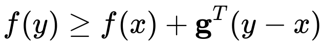
Here, f is the cost function, x is the point where we seek the subgradient, y is any other point in the domain, and g is the subgradient. This condition extends the notion of the tangent line from differentiable functions to non-differentiable convex functions by allowing for any supporting hyperplane that lies below the function graph.

In an optimization scenario (such as subgradient descent), one can pick any valid subgradient at the point of non-differentiability. In practice, deep learning frameworks like PyTorch and TensorFlow often define piecewise gradients for functions like absolute error or hinge loss. Where the function is differentiable, they use the standard derivative. Where the function is not differentiable, they define a subgradient. This piecewise definition allows gradient-based optimization (or subgradient-based optimization) to continue updating model parameters. Although each update may not follow a single “exact” gradient at every kink, the method still converges under conditions similar to those for gradient descent, especially when the learning rate is scheduled appropriately.

In the case of the absolute error function, the slope is -1 when the residual (observed minus predicted) is positive, and +1 when the residual is negative. At the exact point where residual = 0, we can choose any value in the range [-1, 1] as the subgradient. For hinge loss, the function is constant (thus gradient 0) whenever the margin condition is satisfied (yy_hat >= 1) and has a non-zero subgradient (e.g., -y) when the margin is violated (yy_hat < 1). Therefore, through these subgradients or piecewise-defined gradients, backpropagation and other gradient-based methods continue to function even with non-differentiable cost functions.

How Subgradient Descent Works in Practice

In each iteration, the algorithm computes a subgradient g at the current parameter point w. It then updates w by stepping in the negative direction of g, much like standard gradient descent. This step may not exactly align with a steepest descent step if the function is non-differentiable at w, but it still ensures that the parameters move in a direction that can reduce the objective. Over many iterations, with a properly chosen learning rate or an appropriate scheduler, subgradient descent can converge or at least get arbitrarily close to the minimum of a convex function.

Implementation Details in Modern Frameworks

Modern automatic differentiation libraries implement piecewise gradients for these “kinked” functions behind the scenes. When you compute the backward pass, the library essentially decides which piece of the function applies for each data point. This means developers do not usually worry about manually coding subgradients. For example, in PyTorch, the autograd engine has a well-defined subgradient rule for functions like ReLU, absolute value, and hinge-like operations. That is how training pipelines remain smooth even with these functions in the cost.

Potential Follow-up Questions

What is the difference between subgradient and gradient?

Subgradients extend the concept of gradients to functions that lack a well-defined slope everywhere. A gradient is a single vector that uniquely defines the direction of steepest ascent for a differentiable function at a point. In contrast, a subgradient is not necessarily unique at non-differentiable points. Any vector that satisfies the subgradient inequality serves as a valid subgradient. For differentiable points in a convex function, the subgradient coincides with the gradient.

How do we handle a function that is non-smooth in multiple places?

You can define a subgradient for each non-smooth point. For example, in the absolute error function, each absolute value term is piecewise linear with a “kink” at 0. At every point in the domain except at 0, the usual derivative applies. At 0, the subgradient set is [-1, 1]. In practice, frameworks or custom logic detect which side of the kink each term is on and pick an appropriate subgradient.

How does subgradient descent differ from standard gradient descent in terms of convergence properties?

Subgradient descent often requires more careful tuning of the learning rate and typically converges more slowly than gradient descent because the subgradient direction at a kink may not directly correspond to the slope of a smooth function. In some scenarios, it can oscillate around a solution. Convergence can still be guaranteed for convex functions if you use diminishing step sizes or certain adaptive step-size strategies.

What is the role of piecewise-defined gradients in frameworks like TensorFlow or PyTorch?

They implement the rule: where the function is differentiable, use the standard derivative; where it is not, return a valid subgradient. This piecewise approach is often encoded in the symbolic representation of the function, which the automatic differentiation engine parses to build an appropriate computation graph for backpropagation. The frameworks essentially unify the logic of differentiable and non-differentiable segments by internally switching to subgradient-like updates at the kinked regions.

Can non-differentiable functions be optimized just as effectively as differentiable ones?

Many important loss functions, such as L1 regularization, hinge loss, and absolute error, are non-differentiable at some points but are still widely used and optimized in practice. Subgradient methods and piecewise gradient definitions allow gradient-based frameworks to effectively optimize such losses. While the optimization path can be less smooth, it does not usually prevent the algorithm from converging to a suitable solution, especially in large-scale machine learning contexts with ample data.

Below is a short Python code snippet illustrating how subgradient descent on an absolute error loss could be manually implemented. In practice, this is handled automatically by deep learning libraries, but the code helps clarify the concept.

import numpy as np

# Simple example: we want to fit w to minimize sum of |y - w*x|.
# We'll do a few steps of subgradient descent manually.

x = np.array([1.0, 2.0, 3.0, 4.0])
y = np.array([2.0, 4.0, 6.0, 8.0])  # Ideal relationship is y = 2*x
w = 0.0
learning_rate = 0.1

for step in range(10):
    y_pred = w * x
    residual = y - y_pred
    # Subgradient for absolute error: -sign(residual)*x
    # At residual = 0, sign can be anything in [-1,1], choose 0 here for simplicity.
    grad = -np.sign(residual) * x
    grad[residual == 0] = 0.0

    # Average over batch
    grad_mean = np.mean(grad)

    # Update
    w = w - learning_rate * grad_mean

    # Print intermediate results
    print(f"Step {step}: w = {w:.4f}")

This code constructs a trivial linear problem, uses the absolute error, and performs subgradient updates. Although it does not represent how modern libraries do things under the hood (they do it automatically), it demonstrates how subgradients can be handled for non-differentiable costs.

Below are additional follow-up questions

Are subgradient methods guaranteed to converge when the function is not convex?

Subgradient methods, in their classical form, come with strong theoretical convergence guarantees primarily for convex functions. The usual proofs rely on a property called convexity—which ensures that any local minimum is a global minimum, and that subgradient directions are always valid descent directions.

When the function is not convex, the convergence properties become more complicated. In non-convex landscapes, a subgradient step might get stuck in local minima, saddle points, or plateaus, much like standard gradient descent does. Moreover, the set of subgradients at certain kink points might give no clear direction that leads to a global optimum. For instance, if there are multiple “kinks” associated with non-convex structures, different subgradients can point in drastically different directions, making the optimization path highly sensitive to the choice of subgradient.

Nonetheless, in practice—especially in deep learning—people still use “gradient-based” methods on non-convex losses (e.g., piecewise ReLU neural networks). Although formal convergence to a global minimum is not guaranteed, empirical success is often observed. Initialization heuristics, mini-batching, and advanced optimizers like Adam can help escape poor local minima or saddle regions. Still, strictly speaking, one does lose the neat theoretical convergence guarantees that apply in the convex case.

Key pitfalls: • The algorithm can stall in suboptimal regions, showing little improvement in training metrics. • Convergence speed and final performance may heavily depend on hyperparameter scheduling, like the learning rate decay strategy. • Multiple subgradients at a kink can cause abrupt changes in parameter updates, leading to erratic or oscillatory behavior if the function is non-convex.

How do stochastic or mini-batch methods differ from standard subgradient methods for non-differentiable cost functions?

Stochastic and mini-batch variants of subgradient descent update parameters based on a randomly sampled subset of data rather than the full dataset in each step. This approach reduces computation per iteration and often helps with generalization by adding noise to the gradient (or subgradient) estimates. In the context of non-differentiable cost functions, the key difference is that: • You use the subgradient of the sampled data points (or mini-batch) instead of the subgradient of the entire dataset. • This sampling can make the subgradient estimate even more “noisy,” because not only is there a choice among valid subgradients at non-differentiable points, but each mini-batch might yield a different subgradient direction altogether.

Despite the added noise, stochastic subgradient methods remain popular because they can scale to large datasets, and the inherent stochasticity often helps escape local minima or problematic kink regions. The overall convergence properties still depend on convexity for strict proofs, but in practical machine learning, one typically relies on empirical performance rather than pure theory.

Potential pitfalls: • Large variance in subgradient estimates can slow convergence or cause very noisy parameter updates. • Careful mini-batch size selection and learning rate schedules are crucial to mitigate oscillations or divergence. • In extreme cases (very small mini-batch sizes and strongly non-differentiable objectives), training can become unstable if not tuned carefully.

When do we prefer to approximate the non-differentiable function by a smooth surrogate function and what are the trade-offs?

Sometimes, we replace a non-differentiable function with a smooth approximation to exploit standard gradient-based optimization fully. For example, instead of using the absolute value |x|, one might use a differentiable approximation such as sqrt(x^2 + epsilon), or instead of using a hinge loss, one might use a soft-plus function that smoothly approximates the hinge.

We do this in scenarios where: • We want guaranteed differentiability everywhere to apply advanced optimization techniques (e.g., second-order methods or advanced momentum-based optimizers that assume smoothness). • We need smoother gradients for better stability or to avoid abrupt jumps during backpropagation. • We have constraints on hardware or software libraries that require differentiable operations for automatic differentiation or GPU acceleration optimizations.

Trade-offs include: • The surrogate might alter the geometry of the problem, potentially leading to different local minima or solutions that deviate from the original objective. • The approximation may introduce a smoothing parameter that itself must be tuned (epsilon, for instance). • If the smoothing is too strong, you might lose the beneficial properties (like sparsity in the case of L1) that the non-differentiable term was providing. Conversely, too little smoothing might bring you back to the original non-differentiability.

Are there any known issues with vanishing or exploding subgradients for piecewise-defined cost functions like hinge or absolute error?

Vanishing or exploding gradients can occur in almost any gradient-based system, especially when multiple layers or repeated compositions are involved (e.g., deep neural networks). However, piecewise-defined cost functions can accentuate certain issues: • In hinge loss scenarios, if samples are classified “correctly with margin,” the subgradient is zero. This can lead to a vanishing subgradient for large portions of the training data once the model starts to get things right, potentially slowing training because only misclassified or near-boundary examples update the parameters. • In absolute error (L1) scenarios, the subgradient is constant (-1 or +1) away from the kink. This leads neither to a vanishing nor an exploding gradient directly from the cost function itself, but if combined with deep architectures or ill-initialized layers, it can still propagate diminishing or large magnifications of these subgradients across many layers.

Pitfalls in real-world systems: • Once the classifier is doing reasonably well in a hinge-loss setting, few updates might happen, causing the final convergence to be slow. • If intermediate layers amplify or diminish these piecewise gradients in unpredictable ways, you can encounter partial exploding or vanishing behaviors inside the network, particularly with improperly chosen weight initializations or poorly tuned hyperparameters.

How does one handle hyperparameter tuning for subgradient-based methods specifically for non-differentiable objectives?

Hyperparameter tuning for subgradient-based methods can be more challenging because: • Convergence might be more sensitive to learning rate. A too-large learning rate can cause severe oscillations around kink points, preventing stable convergence. A too-small learning rate might stall progress early. • Momentum or adaptive optimizers (like Adam, RMSProp) can behave differently with piecewise gradients, as the directions can abruptly change at kink points, potentially invalidating some momentum assumptions. • Regularization hyperparameters (such as L1 or hinge margin parameters) need to be carefully balanced with the rest of the training setup to avoid overshooting or undershooting.

In practice, you often rely on heuristics like: • Multiple runs with different random seeds to see how consistent the training curves are. • Gradual or piecewise learning rate schedules to handle abrupt gradient changes. • Domain-specific strategies (e.g., focusing on margin violation examples for SVM-like tasks).

A common pitfall is adopting tuning strategies from smooth objectives (like MSE or cross-entropy) and blindly applying them to non-differentiable objectives, leading to suboptimal or erratic training dynamics.

In what scenarios might subgradient descent fail to find a good solution even if the function is convex?

Although subgradient descent has convergence guarantees for convex functions, certain practical factors can cause it to fail to find a suitably good solution: • Learning rate schedules might not be chosen according to theoretical prescriptions (e.g., diminishing step sizes). A fixed learning rate might cause indefinite oscillations. • The function might be convex yet very flat in some directions and steep in others, causing slow progress. • If the subgradients are extremely large or contradictory across different parts of the domain (for instance, with high-variance data), updates can bounce around with no clear path to the optimum. • The presence of constraints (like a constrained convex problem) might create additional complexities when the subgradient points outside the feasible region.

Even though theory tells us subgradient methods should eventually converge for convex objectives, poor practical settings—like an excessively large batch size or not enough iteration budget—could result in an underfit solution.

Could you discuss how the choice of subgradient at a kink point affects the path of optimization, and does it matter in the long run?

When a function is non-differentiable at a kink, there is often an entire set of possible subgradients. For example, in the absolute value function at x=0, any slope in the range [-1, 1] is a valid subgradient. Which subgradient you pick can slightly affect the direction of the update. In practice, frameworks usually follow a convention (often picking 0 for the absolute value at x=0) or a piecewise gradient rule that selects a particular subgradient.

Whether this choice matters significantly over many training steps depends on: • The structure of the loss landscape. In a convex setting, any valid subgradient should theoretically allow subgradient descent to converge given appropriate conditions. • The presence of non-convexities. Different subgradients at kink points can lead to drastically different paths in non-convex scenarios, sometimes resulting in different local minima. • The learning rate schedule. With small enough learning rates or decaying schedules, the path differences introduced by subgradient choices may diminish over time.

Potential pitfalls: • If your chosen subgradient is consistently biased in a certain direction at kink points, it might lead to slower convergence or to a different local optimum in non-convex problems. • In piecewise linear networks or hinge-loss classifiers, repeated encounters with kink points can cause “zig-zagging” if the chosen subgradient changes sign unpredictably.

In many practical machine learning tasks, the difference is often minor compared to larger sources of randomness (like initialization, mini-batch sampling, or data noise). However, for certain sensitive optimization problems, especially smaller-scale or finely tuned scenarios, the subgradient choice at kinks could influence final performance.