ML Interview Q Series: How do gradient-based methods handle relatively flat areas in the optimization landscape, particularly if they contain the target solution?

📚 Browse the full ML Interview series here.

Comprehensive Explanation

Flat regions in the context of gradient-based optimization refer to areas in the loss surface where the gradient is extremely small or practically zero. Since these methods rely heavily on the magnitude and direction of the gradient for making updates to parameters, any region with negligible gradient can slow convergence or lead to ambiguous behavior about which direction to move in.

When we say “flat,” we usually mean the partial derivatives of our cost function are close to zero over a neighborhood of the parameter space. In simpler terms, changes in parameters do not significantly alter the value of the loss in that neighborhood. Sometimes, a flat region may actually represent an entire set of optimal or near-optimal solutions (as in plateaus). Alternatively, the flatness could be a saddle region where curvature is zero along some directions but not others.

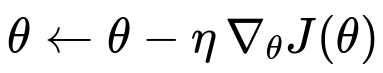
To understand why the gradient matters, consider the standard update rule for gradient descent shown as a central mathematical expression.

Here:

• theta represents the model parameters.

• eta (learning rate) is a positive scalar that controls the step size.

• J(theta) is the loss (or cost) function we aim to minimize.

• nabla_{theta}J(theta) is the gradient of the loss function with respect to the parameters.

If we are in a region where the gradient is very close to zero, the parameter update becomes very small. This can stall learning or make it extremely slow.

Why Flat Regions Occur

Neural networks can exhibit regions where many parameter configurations yield similar or nearly identical loss values. High-dimensional parameter spaces often contain large plateaus or saddle points. Additionally, certain regularized or constrained optimization problems can create extended “valleys” where the loss remains nearly constant.

Common Techniques for Dealing with Flat Regions

Momentum-Based Approaches

Methods like Momentum, Nesterov Accelerated Gradient, and Adam incorporate a moving average of past gradients. This accumulated “velocity” can help the algorithm keep moving even when the instantaneous gradient is small in flat regions. Essentially, momentum helps the optimizer overcome shallow areas by leveraging inertia built from previous gradients.

Adaptive Learning Rates

Optimizers such as RMSProp, Adagrad, and Adam adapt the effective learning rate for each parameter based on recent gradient magnitudes. Parameters that receive consistently small gradients may see their learning rate increase a bit, helping them to continue moving toward a solution in relatively flat regions.

Adding Noise or Stochasticity

Stochastic Gradient Descent already incorporates random sampling of mini-batches. This randomness can help parameters escape flat regions if there is even a slight gradient in some dimension. The noise in the gradient estimate can jiggle the parameters around, giving them a chance to move away from plateaus.

Higher-Order Methods

While not always used in deep learning (due to computational cost), second-order or quasi-Newton methods can detect curvature more accurately. If a region is flat in most directions but not all, second-order approximations can reveal the directions where curvature is nonzero, guiding the parameters toward meaningful descent.

Regularization and Architectural Constraints

In deep neural networks, certain regularizations (like weight decay or weight sharing) and architectural designs (like skip connections in ResNets) can reduce the propensity to get stuck in detrimental flat areas or saddle regions. By shaping the loss landscape, these design choices can also help the model converge to a suitable solution.

How Flat Regions May Actually Be Desired

A flat region of solutions may not always be problematic. Sometimes, it indicates many parameter configurations lead to near-optimal performance. For instance, when the entire plateau corresponds to a very low loss, simply being anywhere on that plateau is acceptable. In practice, small updates in such regions do not harm performance. One can also argue that being in a flatter basin of solutions might improve generalization, as small perturbations in parameters do not drastically change the loss.

Potential Pitfalls

If the region is truly flat, an optimizer might stagnate without a proper mechanism (like momentum or adaptive step sizes) to nudge it out. Also, some methods might interpret a small gradient as a signal to reduce the learning rate further, which might slow progress even more. These subtle effects can lead to confusion about whether the algorithm “converged” or is merely “stuck.”

Follow-Up Questions

What if the plateau is actually the optimal set of solutions? How do we decide on a final solution in that flat region?

In a scenario where an entire plateau corresponds to equally optimal (or near-optimal) solutions, gradient-based methods will typically make infinitesimal updates within that region. This does not harm the model’s performance because all points on that plateau yield similarly good outcomes. In practice, the final solution can be chosen by stopping the training once the overall validation metric stabilizes. Additional constraints or preferences (like model complexity or interpretability) might guide which point in that plateau is ultimately chosen.

How do adaptive learning rate methods help the optimizer navigate flat areas?

Adaptive learning rate algorithms dynamically scale their step sizes based on the history of gradients. When gradients in a particular direction are consistently small, algorithms like RMSProp or Adam can slightly increase the effective step in that direction. This scaling allows the updates to be more noticeable, thus pushing parameters through gentle slopes more effectively than fixed learning rate methods.

Could adding random noise to the gradient estimation really help exit a flat region?

Small random fluctuations in the gradient estimate can jostle the parameters enough to discover a direction with a slight slope. Even if the analytical gradient is exactly zero in some directions, in practice, floating-point precision, batch sampling differences, or data shuffling can yield a non-zero gradient. This can be enough to eventually break free from a near-flat region, particularly in high-dimensional spaces where at least one dimension might have a gentle but non-zero slope.

How do second-order or quasi-Newton methods handle flat regions differently from first-order methods?

Second-order approaches consider curvature by approximating or computing the Hessian matrix (the matrix of second derivatives). Even in a region that appears flat to first-order methods, second-order methods may detect minimal curvature in some directions. By inverting or modifying this Hessian information, they can generate more informative parameter updates. However, the computational and memory overhead often make these methods challenging to scale for very large models.

Are there any tricks to identify if a flat region is a saddle, a plateau, or a local minimum?

One practical approach is to probe the loss landscape in various directions. If the loss remains nearly unchanged in many directions, it might be a plateau. If it increases in some directions and decreases in others, it is more likely a saddle. If it consistently increases in all directions, then it’s a local minimum. In high-dimensional neural networks, exact identification can be expensive, but approximate methods (like Hessian-vector products) or simpler directional checks can offer clues about the nature of the flat area.

When might a flat region be beneficial from a generalization perspective?

Some research suggests that convergence to “wider” or “flatter” minima can promote better generalization because slight parameter perturbations in these regions do not drastically change the output. Conversely, sharper minima can be more sensitive to perturbations. Thus, ending up on a broad flat region of the loss surface can, in many cases, produce a more robust model that performs better on unseen data.

Could you show a minimal code snippet that demonstrates escaping a flat region using an optimizer with momentum?

Below is a simple Python illustration using PyTorch. We define a toy function that has a broad flat region around x=0. Then we use SGD with momentum to see how parameters change.

import torch

# Define a simple function with a flat region around x=0
# For example, f(x) = (x^4) for demonstration: near x=0, the gradient can be very small.
def func(x):
    return x**4

# Parameter initialization
x = torch.tensor([0.1], requires_grad=True)
optimizer = torch.optim.SGD([x], lr=0.01, momentum=0.9)

for step in range(200):
    optimizer.zero_grad()
    loss = func(x)
    loss.backward()
    optimizer.step()

    if step % 20 == 0:
        print(f"Step {step}, x = {x.item():.5f}, loss = {loss.item():.5f}")

In this toy problem, the gradient near x=0 can be quite small, yet the momentum term helps the parameter adjust even in the near-flat region. For real-world deep learning tasks, additional factors (batch noise, larger dimensional spaces, etc.) also help in escaping plateaus.

By carefully tuning optimization hyperparameters and using an appropriate optimizer, gradient-based algorithms can manage flat regions effectively, either by exiting a suboptimal plateau or by settling into a broad region of optimal solutions that generalize well.

Below are additional follow-up questions

What if the learning rate is too high and causes the optimizer to skip over a flat region that is potentially optimal?

A high learning rate can overshadow small gradient signals in near-flat regions. Because updates are scaled by the learning rate, if it is excessively large, the parameter updates can leap across the region rather than steadily moving through it. This might mean missing out on a stable or optimal plateau:

• Potential Pitfall: If the optimization surface contains a broad region of near-optimal values, a large step size might jump entirely over it, settling in a sharper minimum elsewhere or even diverging.

• Real-World Subtlety: In practice, the “optimal” learning rate can vary throughout training. One strategy is to gradually reduce the learning rate as we proceed (learning rate scheduling), ensuring we move quickly in the beginning but carefully explore smaller gradients later.

• Edge Case: When data is noisy or the gradient is stochastic, the learning rate can compound that noise. A large step might bounce out of even a beneficial region. Monitoring loss and validation metrics can be essential to detect such behavior.

If a flat region is very wide, could the gradient appear non-zero but still be too tiny to overcome numerical precision issues?

In very wide plateaus, tiny gradients might be present but smaller than the floating-point precision threshold in practical computation:

• Potential Pitfall: Floating-point underflow or rounding can treat extremely small gradients as zero, thus halting meaningful updates.

• Real-World Subtlety: This is not just a theoretical concern; it can occur in large neural networks when parameter values and gradients span a huge range. Proper initialization and scaling (like batch normalization) can help mitigate extreme gradient values.

• Edge Case: If the network has layers with drastically different magnitude parameters, the gradient calculations for some layers might lose precision entirely. Monitoring gradient norms per layer can uncover this problem.

In very high-dimensional parameter spaces, how can we diagnose if we are stuck in a flat region or merely progressing slowly?

High-dimensional problems often have complex geometry, making it tough to discern true stagnation from slow but steady improvement:

• Potential Pitfall: Looking only at the training loss curve can be misleading; it might plateau briefly before continuing downward at a nearly imperceptible rate.

• Real-World Subtlety: One approach is to track the norm of the gradient. If it remains consistently near zero for many iterations, that strongly suggests a plateau. Alternatively, using multiple random seeds and comparing training trajectories can indicate whether plateaus are a common phenomenon or an artifact of a particular initialization.

• Edge Case: In extremely large models, even if the gradient norm is small, there may exist a sparse but meaningful direction in the parameter space that eventually leads to further descent. Complex model architectures like transformers often hide such directions in their vast parameter manifolds.

Could a flat region near a local minimum cause underfitting?

A flat region could correspond to a suboptimal solution that yields underfitting if the model parameters do not align well with training data patterns:

• Potential Pitfall: Since gradients are small, the optimizer might stay in a suboptimal “valley,” never fully learning the data distribution, resulting in higher training error or poor representation capacity.

• Real-World Subtlety: Even though a local minimum might be stable, it does not mean it is good from a predictive standpoint. This is particularly relevant in smaller datasets or simpler models, where global minima are not guaranteed.

• Edge Case: If the network architecture lacks capacity, even a broad plateau can be the best it can do. Techniques like regularization can sometimes exacerbate this by making the landscape flatter at the expense of fitting complex patterns.

Does increasing the batch size make it easier or harder to escape flat regions?

Batch size can influence the noise in the gradient estimate:

• Potential Pitfall: Larger batches produce more accurate gradient estimates, but with reduced stochastic noise. Less noise can mean slower exploration out of plateaus or shallow regions.

• Real-World Subtlety: In smaller-batch methods, gradient estimates are noisy, but this noise can actually be beneficial for escaping plateaus. Conversely, large-batch training might converge more smoothly but risk getting stuck.

• Edge Case: Extremely large-batch training with limited memory might lead to fewer parameter updates per epoch, further compounding the difficulty in escaping flat regions. Sometimes mixing batch sizes during training (like cyclical or dynamic batch sizes) is used to balance stability and exploration.

Can asynchronous or distributed training dynamics help in maneuvering through flat regions?

In modern large-scale systems, parameters can be updated in parallel across multiple workers:

• Potential Pitfall: If updates are not synchronized properly, stale gradients might interfere with progress and amplify small signals erroneously.

• Real-World Subtlety: When multiple replicas or workers operate on different shards of data, slight differences in updates can push parameters in different directions. This can increase the effective noise, sometimes helping to leave plateaus.

• Edge Case: In extreme cases, too much asynchrony can cause chaotic parameter updates, preventing stable convergence entirely. One might see the loss jump around unpredictably, never settling on a plateau or minimum.

How do initialization strategies affect the likelihood of encountering flat regions?

Parameter initialization sets the starting point, which can heavily influence the optimization path:

• Potential Pitfall: A poor initialization might place the model in an unfavorable flat region that is difficult to escape. This is especially true if the scale of the initial weights is mismatched to the activation functions.

• Real-World Subtlety: Modern techniques like Xavier/Glorot and He initialization aim to keep initial signal variance consistent through layers, reducing the risk of immediate saturation and plateauing.

• Edge Case: In certain architectures with intricate connectivity (like recurrent neural networks), even recommended initializations can lead to vanishing gradients, creating flat-like regions in practice. Specialized initialization or architecture modifications (like LSTM gating mechanisms) may be necessary.

Could adding a small regularization term create or remove flat regions?

Regularization alters the loss landscape by penalizing certain parameter configurations:

• Potential Pitfall: Overly strong regularization can flatten the loss in broad regions if many parameter values produce similarly penalized losses, possibly leading to suboptimal solutions.

• Real-World Subtlety: Conversely, mild regularization can smooth out sharp minima, sometimes making the landscape “flatter” around good solutions, which can improve generalization.

• Edge Case: When combined with constraints (like an L1 penalty that encourages sparsity), regularization might cause the optimizer to get stuck on boundaries in parameter space. In such corners or edges, gradient signals can be abruptly zero in certain parameter directions.

How do skip connections in deep architectures (e.g., ResNets) modify the presence and impact of flat regions?

Skip connections allow gradients to flow more directly through network layers:

• Potential Pitfall: Even with skip connections, certain parts of the network can have near-flat gradients if those parameters do not significantly affect the final output. This can occur in sub-blocks that the skip bypasses heavily.

• Real-World Subtlety: Generally, skip connections improve the condition of the loss landscape by reducing vanishing gradients, thereby diminishing the size of flat regions that hamper training. However, they do not eliminate all potential flatness; some layers can still have minimal gradients if the forward signal does not rely much on those layers.

• Edge Case: In very deep networks with skip connections, some subtle interactions between the skip pathways and main pathways may create partial plateaus. The training might move faster in skip-connected layers while slower in deeper or more convoluted substructures.

Could overparameterization (e.g., extremely large models) make flat regions more common?

Modern deep networks often have orders of magnitude more parameters than training examples:

• Potential Pitfall: Overparameterization can indeed lead to extensive manifolds of nearly identical solutions, effectively expanding the size of flat regions.

• Real-World Subtlety: Although overparameterization can help models achieve very low training error, it also raises questions about how well the model generalizes. Large networks might converge to a broad, flat area but require careful regularization or early stopping to avoid overfitting.

• Edge Case: Extremely overparameterized networks may show nearly zero gradient for many parameters while some critical subset of parameters does the main “heavy lifting.” Identifying these crucial parameters can be challenging and might require techniques like pruning or lottery ticket hypothesis approaches.

Could catastrophic forgetting in continual learning be related to getting stuck in or leaving a flat region?

In continual learning, a model learns new tasks sequentially and often forgets previously learned tasks:

• Potential Pitfall: When shifting to a new task, if the previously learned parameters lie in a flat region for the old task’s loss, updates from the new task can move the model out of that plateau, negatively impacting old-task performance.

• Real-World Subtlety: Techniques like Elastic Weight Consolidation try to penalize moves away from important parameters for old tasks. This effectively shapes the loss landscape to keep the model in a flatter region that satisfies multiple tasks. Yet, if that region is not truly optimal for either task, it can lead to underperformance in both.

• Edge Case: If the tasks conflict strongly, no common flat region may exist that satisfies all tasks. The optimizer might bounce between partial plateaus for each task, failing to fully converge on a stable solution.