ML Interview Q Series: How do k-Means and k-Nearest Neighbors fundamentally differ in their approach and purpose?

📚 Browse the full ML Interview series here.

Comprehensive Explanation

k-Means and k-Nearest Neighbors (kNN) are frequently confused due to their similar naming and the presence of the parameter k in each. However, the two algorithms serve entirely different purposes and operate under distinct paradigms.

High-Level Overview

k-Means is an unsupervised clustering algorithm. It attempts to find structure in unlabeled data by partitioning data points into k clusters such that each point belongs to the cluster with the nearest mean. The means (or centroids) are iteratively updated to minimize the overall distance of points within each cluster.

k-Nearest Neighbors is a supervised learning method. It relies on a labeled dataset and assigns the label of a new sample based on the labels of the k closest points from the training data. In classification tasks, the class is typically decided by majority vote among the k nearest labeled points, while in regression tasks, the outcome is often taken as the average of those neighbors’ numeric values.

k-Means Core Objective

At the heart of k-Means is an objective function that tries to minimize the sum of squared distances between data points and their cluster centroids.

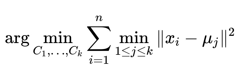
Here n is the number of data points, x_i denotes the ith data point in your dataset, k is the number of clusters, and mu_j (the jth centroid) is the mean of all points assigned to cluster j. Minimizing this sum of squared distances leads to more compact clusters in the feature space. The algorithm works by alternating between two key steps: • Assignment step: Assign each data point to the nearest centroid. • Update step: Recalculate each centroid as the mean of points currently assigned to that cluster.

k-Nearest Neighbors Core Idea

In kNN, there is no iterative “training” phase in the traditional sense, which makes it a lazy learner. The decision for a new data point x depends on identifying its k closest neighbors in the training set. If the task is classification, the class is decided by a majority vote among those neighbors. If the task is regression, the prediction is typically the average value of those neighbors’ target values. Distance is often measured using Euclidean distance, although other metrics like Manhattan distance or Minkowski distance can be used.

Purpose and Supervision

k-Means is unsupervised: It only tries to group unlabeled data into clusters. You do not have any labels; you simply want to discover some intrinsic groupings in the data.

kNN is supervised: It requires labeled training data to decide how to label new, unseen data points. If there are no labels in the training set, kNN cannot assign a label to a new point.

Usage Scenarios

• k-Means is appropriate when you want to discover underlying structures in unlabeled data or reduce the dimensionality of data (after forming clusters, sometimes clusters can be used as a new categorical feature). • kNN is useful when you have labeled data and want to classify or perform regression on new data points. It can be a good baseline method because of its simplicity.

Complexity and Practical Considerations

For k-Means: • The algorithm can converge to local minima, so initialization of centroids can matter (e.g., k-means++ initialization helps). • You need to choose k, the number of clusters, often by heuristics like the “elbow method.” • Complexity for each iteration is typically O(n * k * d), where d is the dimension of the data, because you compute the distance to k centroids for n data points.

For kNN: • The algorithm can be expensive during prediction, because it must compute distance from the query point to potentially all points in the training dataset. • You need to choose k, the number of neighbors, which can significantly impact bias-variance trade-offs. • Storing the training data is mandatory; memory usage can be high if the training set is large. Some structures like KD-trees or Ball Trees can speed up neighbor searches.

Example Code Snippets

Below is a simple Python snippet using scikit-learn for k-Means:

from sklearn.cluster import KMeans
import numpy as np

# Suppose X is your unlabeled data
X = np.array([
    [1, 2],
    [1, 4],
    [5, 6],
    [6, 7],
    [2, 3]
])

kmeans = KMeans(n_clusters=2, random_state=0).fit(X)
print("Cluster assignments:", kmeans.labels_)
print("Centroids:", kmeans.cluster_centers_)

And a quick example for kNN classification with scikit-learn:

from sklearn.neighbors import KNeighborsClassifier
import numpy as np

# Suppose X is your training data, y are labels
X = np.array([
    [1, 2],
    [1, 4],
    [5, 6],
    [6, 7],
    [2, 3]
])
y = np.array([0, 0, 1, 1, 0])  # some labels

knn = KNeighborsClassifier(n_neighbors=3)
knn.fit(X, y)

test_point = np.array([[2, 4]])
prediction = knn.predict(test_point)
print("Predicted class:", prediction)

Why They Are Confused

Both have the parameter k, and both rely on the notion of distances in a feature space. However, k-Means focuses on grouping unlabeled data into k clusters, while kNN focuses on using a labeled dataset to predict an unknown sample’s label based on the majority or average label of its k nearest neighbors.

Potential Follow-up Questions

How do you choose k in k-Means and kNN differently?

Choosing k in k-Means often involves domain knowledge or heuristic methods. One common approach is the “elbow method,” where you run k-Means for various k values and observe how the sum of within-cluster variance decreases. You look for a point where the rate of decrease sharply changes (forming an elbow shape on a plot).

In kNN, k is chosen by considering accuracy on a validation set or through cross-validation. Low k can lead to high variance (overfitting), while high k can introduce bias (underfitting). A typical strategy is to test multiple k values, pick the one yielding the best performance on validation data.

How does the distance metric affect both algorithms?

In k-Means, the standard distance metric is Euclidean distance. Using different metrics changes what “center” or “mean” might represent. Though uncommon, some variations of k-Means adapt the concept of distance differently.

In kNN, the choice of distance metric can drastically affect neighbor relationships. Euclidean distance is the most standard, but Manhattan or other distance functions are used when the feature space or domain suggests it. For instance, if features represent geographical blocks in a city, Manhattan distance might be more meaningful.

When would you not use kNN for a classification problem?

kNN becomes impractical when the dataset is extremely large, because finding neighbors can be computationally expensive. It also performs poorly in high-dimensional spaces (the curse of dimensionality makes distances less meaningful). If real-time prediction speed is crucial and you have very large training data, a more efficient classifier such as a support vector machine or a random forest may be a better choice.

Can k-Means handle non-spherical clusters?

k-Means inherently favors spherical or convex clusters, as it relies on distances to centroids. In data where clusters are elongated, have varying densities, or are otherwise non-convex, k-Means may struggle. Alternative methods like DBSCAN or Gaussian Mixture Models might be more suitable if cluster shapes are irregular or if you expect varying densities.

Are there any common pitfalls to watch out for with either approach?

One common pitfall in k-Means is poor centroid initialization leading to suboptimal clustering. Using smarter initialization (k-means++) or performing multiple runs can mitigate this. Another issue is the assumption that each cluster is roughly spherical and has roughly equal variance.

A pitfall in kNN is the sensitivity to irrelevant or unscaled features. Feature scaling (for example, normalization or standardization) can significantly improve performance. Also, having noisy or mislabeled data points in the training set can directly affect predictions since kNN uses actual labeled instances to vote on the class or regression value.

Both algorithms can be heavily impacted by outliers, so care must be taken with data cleaning and normalization.

Below are additional follow-up questions

How does feature scaling or normalization impact both k-Means and kNN?

Feature scaling can significantly affect both algorithms, but in different ways. For k-Means, distance calculations determine cluster assignments. If one feature has a large range of values while others are small, then that dominant feature might overshadow the distances in lower-scale features, causing clusters to be driven primarily by the higher-scale dimension. Normalizing or standardizing features (for instance, subtracting the mean and dividing by the standard deviation) helps ensure that no single dimension disproportionately influences the distance metric in k-Means.

In kNN, the same pitfall can occur. The nearest neighbors are chosen based on distance computations, so if one feature spans a much larger numerical range, then it can dominate the distance metric. By scaling all features, each dimension contributes more fairly to the neighbor selection process. Without scaling, especially when different features come from distinct domains (e.g., age vs. income vs. text embeddings), the unnormalized features can skew the results of kNN classification or regression.

Edge cases: • If a dataset has a single feature with a massive range (such as annual income reaching the millions) and other features that vary in a small range (like 0-10), then ignoring feature scaling might cause the algorithms to cluster or classify almost entirely based on that single large-range feature. • Too-aggressive scaling can also be a pitfall in cases where domain knowledge actually suggests that certain features should weigh more heavily than others.

What happens if the dataset for k-Means has extreme outliers?

In k-Means, outliers can severely affect cluster centroids because centroids are calculated by averaging the positions of the points in each cluster. If there is even a single extreme outlier in a cluster, the centroid can shift drastically toward that point. This can degrade the overall clustering quality, as one cluster might get skewed due to the outlier. Furthermore, if outliers appear in the data, it can cause the sum of squared distances to spike, which often leads to suboptimal results.

Possible mitigation strategies include: • Using robust clustering variants such as k-Medoids, which relies on choosing actual data points as centers rather than means, making it less sensitive to extreme outliers. • Applying outlier detection methods in a preprocessing step, then removing those identified outliers from the dataset before clustering. • Employing data transformations (for example, log transformations if the data is heavily skewed in certain dimensions) to reduce the impact of extreme values.

Edge cases: • A small number of legitimate but extreme data points could represent a niche user group or rare event. Removing them blindly might lose critical information about that unique subgroup. Thus, domain knowledge should guide outlier handling. • Clusters can sometimes be too fragmented if outliers remain, leading to poor interpretability when each cluster’s centroid is disproportionately pulled away from the majority of points.

In what ways can we evaluate the results of k-Means clustering versus a supervised algorithm like kNN?

Because k-Means is unsupervised, common evaluation metrics include inertia (sum of squared distances to centroids), silhouette score (how similar each point is to its assigned cluster compared to other clusters), and Calinski-Harabasz or Davies-Bouldin indices. These measures rely on intrinsic properties of the data and how well they group together, as there are no true labels to compare against.

By contrast, kNN is typically evaluated using supervised learning metrics like accuracy, precision, recall, F1-score for classification tasks, or mean squared error (MSE), mean absolute error (MAE), or R^2 for regression tasks. Because kNN predictions can be compared against ground-truth labels, the evaluation is more direct.

Edge cases: • When evaluating k-Means, one might try to retroactively label the clusters and measure performance, but unless true labels are known, it becomes guesswork. If partial labels are available, or if a domain-expert labeling is done post hoc, evaluation becomes a bit more supervised. • In kNN, a small test set might lead to misleading evaluation metrics if the dataset is not representative. Cross-validation or stratified sampling can mitigate this issue, especially when certain classes are rare.

How do categorical features affect k-Means versus kNN?

k-Means requires a notion of “mean” for computing centroids, so it naturally fits continuous numeric data. Incorporating categorical variables is tricky because you cannot simply take an arithmetic mean of categories. One workaround might be one-hot encoding or dummy variables, but then each category is turned into a binary dimension. The Euclidean distance in such a high-dimensional binary space is not always meaningful, and the algorithm might be skewed if some categories are rare.

kNN can handle categorical variables more flexibly, as the distance can be defined in other ways. For instance, one could use Hamming distance for binary attributes (counts the number of positions at which the corresponding values differ). Alternatively, you can encode the categorical feature as ordinal or via embeddings, then rely on a more conventional distance metric. Still, if the number of categories is large and simply one-hot encoded, the dimensionality can become huge, and kNN may become less effective.

Edge cases: • In k-Means, mixing numeric and categorical data can produce clusters that are not interpretable. Clusters might be heavily dominated by numeric features while categorical dimensions add noise, or vice versa. • In kNN, if a single categorical feature has many possible categories (e.g., thousands of product types), naive one-hot encoding can inflate dimensionality and degrade performance significantly.

How do k-Means and kNN scale to very large datasets in practice?

k-Means often scales relatively well with large datasets, but the algorithm might still require multiple passes over the dataset to refine clusters. Techniques like mini-batch k-Means process data in small batches, updating centroids incrementally. This reduces memory usage and can speed up the process for massive datasets.

kNN’s prediction phase can become a bottleneck because every new query requires calculating the distance to a large subset (or the entire set) of training points. This cost grows linearly with the size of the training set unless specialized data structures (like KD-Trees or Ball Trees) are used. Even then, in very high dimensions, these structures might not offer significant speedups. Approximate nearest neighbor methods can mitigate this issue by trading off a small loss in accuracy for a significant gain in query speed.

Edge cases: • In streaming or online scenarios, k-Means with mini-batches might be feasible for continuous updates, but kNN has limited ability to handle streams unless you employ window-based approaches (where you discard older data) or keep some form of dynamic data structure. • If the dataset is extremely sparse and high-dimensional (such as text data in NLP), both k-Means and kNN might require specialized techniques or dimension-reduction methods like PCA or truncated SVD to handle computational complexity and memory constraints.

When would you consider using soft clustering methods (like Gaussian Mixture Models) instead of k-Means, and how is that different from switching to kNN?

k-Means performs hard clustering: each point definitively belongs to exactly one cluster. However, there are cases where a data point could sensibly belong to more than one cluster to varying degrees—this is where Gaussian Mixture Models (GMM) can shine. GMMs assign probabilities of cluster membership rather than a single membership. This probabilistic framework can capture uncertainty and more flexible cluster shapes (elliptical in the feature space).

Switching to kNN is a different choice entirely. If you have labels and want a supervised method to classify new points, kNN is one straightforward approach. Soft clustering, on the other hand, is still typically unsupervised (though semi-supervised variations exist) and aims to capture the underlying structure of unlabeled data. If your goal is classification or regression with labeled data, kNN might be relevant. If your goal is to cluster data that may belong to multiple overlapping clusters, a soft clustering method like GMM is typically better.

Edge cases: • If you attempt to adapt kNN to a scenario where data might not have discrete class boundaries (e.g., fuzzy classes in certain biological or marketing applications), you might end up with uncertain or conflicting nearest neighbors. Soft clustering provides a more direct probabilistic mechanism for partial memberships. • GMM can be computationally more expensive and also more sensitive to initialization. If the number of mixture components is large or the feature space is high-dimensional, training could be slow or converge to suboptimal solutions.

What are the considerations if we want to use clusters from k-Means as features for another supervised algorithm, and how does that compare to using kNN output as features?

Sometimes, after performing k-Means, you might use the cluster membership or cluster distances as a feature in a downstream supervised model. For instance, you can add an indicator feature representing which cluster each data point belongs to, or you can include the distance of the point to each cluster centroid as additional input features. This approach can reveal latent groupings in your data that might enhance a subsequent classification or regression model.

Using kNN output as features is less common because kNN is a lazy learner that does not produce a compact, learned representation. You could, in theory, augment data with “the label distribution of the k nearest neighbors,” but that tends to be more of a meta-learning approach than a typical practice. More commonly, you might use distances to a subset of prototypes (sometimes known as a nearest prototype approach) as features. However, that starts to resemble methods like learning vector quantization (LVQ) rather than standard kNN.

Edge cases: • When using k-Means cluster assignments as features, it is essential to consider that these clusters were derived in an unsupervised manner. The discovered clusters might not align perfectly with the supervised objective. Sometimes you get “pure clusters” that map well to actual classes or real-world segments, and sometimes the clusters mix labels, adding little value. • If you change the number of clusters k drastically, it can produce a high-dimensional indicator feature that might require additional feature selection or regularization in the downstream model.

How does the concept of decision boundaries differ between k-Means (if we treat cluster index as a label) and kNN in a supervised setting?

If you artificially treat each cluster from k-Means as a label, you effectively create regions in the feature space where the data is closer to a certain centroid than any other. These boundaries are constructed based on Voronoi partitions around the centroids. The centroid positions define where the boundaries lie, and each data point falls into the nearest centroid’s region.

In kNN, the decision boundary is formed by the local neighborhood structure of the training data. Unlike k-Means, which has a fixed set of k global centroids, kNN’s “boundary” is collectively influenced by the positions and labels of potentially all training points. As you move through the feature space, a region is assigned to a particular label when the majority of points in that region’s local neighborhood share that label.

Edge cases: • If clusters are not well-separated in k-Means, the boundaries might slice across dense regions of data that truly belong to multiple classes, especially if the data was unlabeled. • In kNN, noisy labeling or uneven label distributions can produce jagged or fragmented boundaries. A small number of mislabeled points in a dense region can shift the majority vote near the boundary.