
ML Interview Q Series: How do negative sampling approaches in word2vec or related embedding methods serve as a form of cost function design, and why might full softmax be impractical?

📚 Browse the full ML Interview series here.
Hint: Negative sampling drastically reduces computation by sampling only a few negative classes.
Comprehensive Explanation
Negative sampling is a technique introduced in word2vec and related methods that frames embedding training as a simpler classification problem rather than performing a full softmax over a large vocabulary. In typical word embedding frameworks like the skip-gram architecture, the training objective is to predict a target word given a context word (or vice versa). Doing a full softmax over all possible target words can be extremely costly when the vocabulary is large (e.g., tens or hundreds of thousands of tokens). Negative sampling replaces this expensive normalization step with a small logistic classification task: for a given (context, target) pair, the model is trained to distinguish it from randomly sampled “negative” pairs.
When performing negative sampling, we typically pick a few negative words (e.g., 5 to 20) according to some distribution (often proportional to the unigram frequency raised to the 3/4 power). Then, for each actual (context, target) pair, the model is pushed to increase the similarity between the corresponding embeddings, while simultaneously decreasing the similarity between the embeddings of the context and the negative samples.
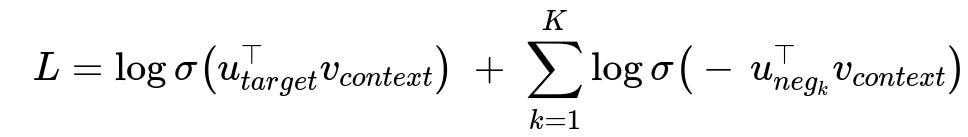
Below is the typical negative sampling objective for a single positive (context, target) pair, plus K negative samples. The central formula often used in the skip-gram model with negative sampling is shown here.
Parameters:
u_{target}is the embedding of the target word.v_{context}is the embedding of the context word.u_{neg_k}is the embedding of the k-th negative word.Kis the number of negative samples.The function
sigma(x)is the logistic sigmoid function 1 / (1 + e^(-x)).
This approach treats the training as a binary classification task: the model wants to output a high probability for (context, target) being a true pair and a low probability for (context, negative) being a true pair. Each term in the loss is a log-likelihood under the assumption that the positive pair should yield a label of 1, while negative pairs yield a label of 0. It avoids computing a normalization constant across the entire vocabulary, which would otherwise be required for a full softmax.
Why full softmax is impractical
For a large vocabulary, doing a full softmax means computing unnormalized scores (logits) for every word in the vocabulary and then computing the softmax denominator as the sum of the exponentials of those scores. This can be very expensive when the vocabulary can be tens of thousands or even millions of words. Negative sampling circumvents the need to compute these scores for all words by only sampling a handful of negative examples per positive training pair. This drastically reduces computational overhead.
Practical Implementation Aspects
In many frameworks (like word2vec and other embedding methods), negative sampling is the default choice for training because it is both memory-efficient and computationally efficient. When we implement it, we:
Maintain a distribution for sampling negative words (often proportional to word frequency raised to 3/4).
For every (context, target) pair, draw K negative words from this distribution.
Compute the binary logistic loss for the positive pair and the negative pairs.
Update the embeddings via backpropagation.
A sample implementation in Python (using a pseudo-PyTorch-like style) could look like this:
import torch
import torch.nn.functional as F

class SimpleEmbeddingModel(torch.nn.Module):
    def __init__(self, vocab_size, embedding_dim):
        super().__init__()
        self.in_embeddings = torch.nn.Embedding(vocab_size, embedding_dim)
        self.out_embeddings = torch.nn.Embedding(vocab_size, embedding_dim)

    def forward(self, context_indices, target_indices, negative_indices):
        # context_indices: (batch_size,)
        # target_indices: (batch_size,)
        # negative_indices: (batch_size, K)

        v_context = self.in_embeddings(context_indices)       # (batch_size, embedding_dim)
        u_target = self.out_embeddings(target_indices)        # (batch_size, embedding_dim)
        u_negatives = self.out_embeddings(negative_indices)   # (batch_size, K, embedding_dim)

        # Positive scores
        pos_scores = torch.sum(v_context * u_target, dim=1)  # (batch_size,)
        pos_loss = F.logsigmoid(pos_scores)

        # Negative scores
        neg_scores = torch.bmm(u_negatives, v_context.unsqueeze(2)).squeeze(2)  # (batch_size, K)
        neg_loss = F.logsigmoid(-neg_scores).sum(dim=1)

        # Total loss
        total_loss = -(pos_loss + neg_loss).mean()
        return total_loss
In this simplified snippet, we compute the dot product between the context embedding and the target embedding for the positive pair, and we compute the dot product between the context embedding and each of the negative word embeddings for the negative samples. We then apply the log-sigmoid (logistic) function. The negative samples are forced to have low dot product with the context, while the correct target word is forced to have a high dot product.
Follow-up Question 1
Why do we prefer negative sampling over hierarchical softmax in practice?
Negative sampling is often simpler to implement and can be faster when dealing with only a small number of negative examples. Hierarchical softmax uses a binary tree to compute the full distribution more efficiently, but it still has overhead related to tree depth and additional structures. Negative sampling, on the other hand, trades off a tiny bit of accuracy for a massive speed gain and is typically easier to parallelize. Additionally, negative sampling can yield better empirical results for word embeddings because it consistently focuses on discriminating a small set of negative words from the positive one, which can be beneficial if that small set is frequently sampled from a meaningful distribution.
Follow-up Question 2
How do we choose the distribution from which to sample negative words?
A common heuristic is to sample words from a distribution proportional to their unigram frequency raised to the 3/4 power. In text form, we might say p(word) ∝ (frequency(word))^(3/4). This slightly downweights very frequent words while still allowing them to appear often enough as negatives. This helps maintain a good balance where extremely frequent words are not always chosen, but also not so rare that the model never sees them as negative examples.
Follow-up Question 3
What is the difference between negative sampling and noise-contrastive estimation (NCE)?
Noise-contrastive estimation (NCE) is more general: it tries to fit the model’s distribution to a target distribution (like the true word distribution) by comparing real data to artificially generated noise. Negative sampling can be viewed as a simplified variant of NCE specifically designed for word embedding tasks, where the number of negative samples and logistic loss objective are tailored for embeddings. NCE explicitly learns normalization constants, while negative sampling omits the full normalization factor. In practice, negative sampling is a special-case approach that is easy to implement and known to perform extremely well for word embedding training.
Follow-up Question 4
What happens if we choose too few or too many negative samples?
Choosing too few negative samples (like K=1) might not give enough discrimination power to the model, causing underfitting or insufficient gradient signal. Choosing too many negative samples unnecessarily increases computation time and might lead to overemphasizing the discrimination of negatives relative to the correct positive. Empirically, a moderate number (5–20) often achieves a good balance, though the “best” choice depends on the dataset size, model architecture, and training budget.
Follow-up Question 5
How does negative sampling handle rare words versus frequent words?
Rare words are less likely to appear as negative samples because they have low sampling probability. However, when they do appear in actual context-target pairs, the model focuses on learning meaningful embeddings through the positive training signal. Frequent words appear more often both as positive and negative samples, which can accelerate learning for the most common words and ensure they are well-positioned in the embedding space. The 3/4 power heuristic is especially designed to adjust the distribution so that some moderately frequent words appear often enough, but extremely frequent words are not overwhelmingly chosen.
Follow-up Question 6
Could negative sampling degrade model performance if not used properly?
Yes. If the negative sampling distribution is poorly chosen, or if the number of negative samples is too large or too small, the quality of the learned embeddings can suffer. Also, in domains where the vocabulary is smaller, or where the distribution is highly skewed, one might want to consider techniques like hierarchical softmax or even full softmax if the vocabulary is not massive. Negative sampling is extremely powerful for large vocabularies, but it must be tuned with the right sampling distribution and number of negatives to maintain good performance.
Below are additional follow-up questions
Could negative sampling lead to data imbalance issues and how might we address them?
Negative sampling could skew the training distribution if the same frequent words are sampled disproportionately often as negatives. This might cause the model to over-reinforce discrimination against certain words while neglecting others. In typical text corpora, frequent words are already quite prevalent, so sampling them at an even higher rate can exacerbate imbalance. One way to address this is to adjust the sampling distribution (e.g., raising frequencies to the 3/4 power) so the extremely frequent words do not dominate the negative set. Another approach is to combine dynamic sampling strategies (e.g., adaptively adjusting negative sample probabilities based on model performance) to ensure a more balanced representation of the vocabulary. In rare data domains with heavy skew (like specialized medical terminologies where a few tokens dominate), it may be necessary to design a custom sampling heuristic (for instance, capping the maximum sampling probability of extremely frequent tokens).
How does negative sampling integrate with subword embeddings (e.g., fastText), and what unique pitfalls arise?
When using subword or character n-gram embeddings (like fastText), each word vector is actually composed of multiple subword vectors. Negative sampling still applies, but we must consider the subword representation at training time. For instance, if the context word is “running,” the model might combine n-gram embeddings such as “runn,” “unni,” “ning,” etc. A subtle pitfall is that frequent subwords (like common prefixes or suffixes) might appear as part of multiple sampled negatives across different words, increasing the gradient updates applied to their embeddings. If these subwords dominate the training signal, the model may fail to learn more specialized n-gram representations. One strategy to mitigate this is to ensure that negative subword fragments are also sampled proportionally or to incorporate frequency thresholds so that extremely common subwords do not overwhelm the updates.
How can repeated sampling of the same negative examples affect the training dynamics?
If the same negative examples are sampled repeatedly for a particular (context, target) pair, the model might “over-learn” to discriminate that specific set of negatives while not generalizing well to others. This can happen if the random seed or sampling distribution is not well-shuffled or if a small subset of words consistently shows up as negatives. The model would become very good at telling the difference between the true target and that small set of negatives, but might not adequately learn to discriminate the target word from a broader range of vocabulary. One potential solution is to use large shuffle buffers or to ensure each context-target pair sees a diverse set of negatives across epochs. Setting a sufficiently large negative sample size distribution can also help reduce the likelihood of repeated samples within the same mini-batch or across consecutive batches.
Is negative sampling guaranteed to find a globally optimal set of embeddings?
Like most neural network training approaches, negative sampling is not guaranteed to converge to a global optimum. Stochastic gradient-based methods can get stuck in local optima or saddle points, especially with high-dimensional embeddings. The effectiveness of negative sampling also depends on the sampling distribution, the learning rate schedule, and the initialization of embeddings. In many practical scenarios, the method converges to a sufficiently good local minimum that yields high-quality embeddings. Empirically, negative sampling has shown strong performance despite the lack of formal global optimality guarantees. Careful tuning of hyperparameters (like the number of negatives, learning rate decay, and the sampling distribution exponent) can help steer the model toward more stable minima.
Are there scenarios where full softmax or hierarchical softmax might outperform negative sampling?
If the vocabulary is relatively small, or if complete probability distributions over words are necessary for downstream tasks, then full softmax or hierarchical softmax can be more appropriate. Negative sampling does not directly produce normalized probabilities over the vocabulary; it focuses on pairwise discrimination. If a language model or an application explicitly requires normalized word likelihoods, negative sampling might require an additional correction or might not be the ideal approach. In smaller vocabularies, the computational advantage of negative sampling diminishes, so hierarchical softmax or even full softmax can be practical. Another scenario is if interpretability of the predicted word probabilities is critical, in which case negative sampling’s unnormalized approach is less straightforward to interpret.
How might negative sampling be extended or adapted beyond word-level embeddings to handle phrases or sentences?
When embedding phrases or sentences (e.g., in sentence embedding tasks), negative sampling can still be used if we treat the phrase or sentence as the “target” instead of a single word. For instance, in a sentence embedding framework, we might sample unrelated sentences as negatives. The pitfall here is increased complexity in deciding how to generate negative examples. Randomly picking sentences from the corpus might be too easy for the model to discriminate, leading to insufficient gradient signal. One might sample negative sentences that are syntactically or semantically similar but not identical, creating a more challenging (context, negative) contrast. This design can be more intricate, because measuring similarity at the sentence level requires either heuristic or learned metrics, and an ill-chosen strategy could degrade the quality of the learned embeddings by focusing on trivial or overly difficult negatives.
What are potential memory or computational bottlenecks when implementing negative sampling in large-scale systems?
Even though negative sampling is generally more efficient than full softmax, it can still become a bottleneck if the vocabulary is huge. Storing, shuffling, and sampling from a large vocabulary requires efficient data structures. For instance, a high-performance reservoir or a rolling buffer might be necessary. On distributed systems, synchronization overhead or uneven distribution of word frequencies can lead to imbalanced workloads. Additionally, each negative sample requires a separate embedding lookup and gradient update, which can strain memory bandwidth. One practical solution is to batch embeddings lookups carefully or precompute subsets of popular negative words for faster sampling on GPUs. Another trick is caching frequently used embeddings in faster memory layers or using approximate nearest neighbor structures to pick negatives.
Can negative sampling be used for tasks beyond language modeling, and what special considerations might arise?
Yes, negative sampling is used in recommender systems (e.g., to distinguish a user’s clicked items from random non-clicked items), knowledge graph embeddings (to distinguish true relational facts from negative triples), and even image similarity tasks. Special considerations include how to define a “negative sample” in domains outside of text. For instance, in a knowledge graph, we might replace a head or tail entity with a random entity to generate a negative triple. If the sampling distribution is not carefully chosen—say, sampling invalid entities that never appear in certain contexts—this could lead to trivial negatives that provide little training signal. Balancing the frequency of different entity or item types is crucial so that the model does not become biased toward easily discriminable negatives.
How might dynamic negative sampling strategies improve training?
In dynamic negative sampling, the model adaptively selects “hard negatives” that are close to the correct target in embedding space. Early in training, random negatives might suffice, but as the model improves, it becomes easy for it to distinguish random negatives, resulting in less useful gradient signals. A dynamic or hard-negative approach continually updates a priority queue of potential negatives based on their similarity scores to the context. This strategy can accelerate learning by focusing on the negatives that the model finds most confusing. The trade-off is higher computational cost for repeatedly identifying and sampling these hard negatives. There is also a risk of reinforcing spurious similarities if the sampling focuses too heavily on a small set of ambiguous negatives, so careful calibration is needed.