ML Interview Q Series: How do normalisation and standardisation differ in data preprocessing?

Comprehensive Explanation

Normalisation usually aims to rescale data so that all values lie within a fixed range, commonly 0 to 1. Standardisation, on the other hand, transforms the distribution of the data so that it has a mean of 0 and a standard deviation of 1. Both methods alter the distribution of features in different ways, and each is suited to different contexts.

One of the most frequently used normalisation approaches is min-max scaling, which takes each data value and subtracts the minimum value of the feature, then divides by the range. The main purpose is to confine the values of a feature to a bounding interval, ensuring that no feature dominates simply by virtue of its numeric range.

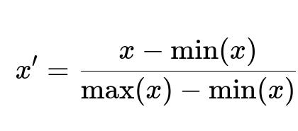
Here, x is the original data point, min(x) is the smallest value of the feature in the dataset, and max(x) is the largest value of the feature in the dataset. This formula repositions and stretches or shrinks the data so that the smallest value becomes 0, the largest value becomes 1, and all other values lie proportionally in between.

Standardisation, in contrast, modifies the data such that it has zero mean and unit variance. The result of standardisation is often used in algorithms that assume normally distributed data or that are sensitive to differences in scale among features.

Here, x is the data point, mu is the mean of the feature, and sigma is the standard deviation of that feature. The transformation moves the center of the data to 0 (by subtracting mu), then normalises the spread (by dividing by sigma). As a result, most of the data in a normally distributed feature will fit between -3 and +3.

Both methods serve to reduce disproportionate influence of features that naturally have large values. However, normalisation preserves a clear boundary and shape relative to a fixed range, while standardisation re-centers the distribution around 0 and ensures it has a variance of 1.

In practice, normalisation is often helpful for distance-based algorithms such as k-Nearest Neighbors, or neural networks with certain activation functions that perform best within a limited numeric range. Standardisation is widely used for linear models like logistic regression or support vector machines, which depend on data shaped around mean 0 for stable convergence. Outliers can significantly affect min-max scaling, since the range might become very large, whereas standardisation is somewhat more robust to moderate outliers (though it can still be affected if extreme values cause a large standard deviation).

How do outliers affect these transformations differently?

Outliers can shift the range of a feature and thus squash most of the values in min-max scaling. If the maximum value is unusually large, the normalised data for the rest of the points can collapse near 0. Standardisation also reacts to outliers because an extreme data point can drive up the standard deviation, though the effect is often less severe compared to min-max normalisation. Nonetheless, in the presence of extreme outliers, even standardisation might not be sufficient, and techniques like robust scaling (based on interquartile range) can offer a more stable transformation.

When might normalisation be preferred over standardisation?

Normalisation can be advantageous when you want to constrain your data values to a fixed interval, such as when feeding inputs to certain neural networks that assume data lies within 0 and 1. It is also helpful in scenarios like image processing, where pixel values are typically normalised to speed up and stabilise training. Distance-based algorithms, such as k-Nearest Neighbors, often operate more effectively on data that is scaled to a specific range, so that no single feature with large numeric values overwhelms distance calculations.

When might standardisation be the better choice?

Standardisation is often the go-to option for algorithms that assume a Gaussian-like distribution. Linear and logistic regression, support vector machines, and principal component analysis often converge more quickly and produce more reliable results when features have zero mean and unit variance. Furthermore, if the data is already approximately normal, standardisation helps maintain that shape, simply shifting and scaling it in a way that can benefit these models.

Does the choice depend on data distribution?

If a feature is heavily skewed or has many outliers, normalisation or standardisation alone might not suffice. In such cases, log transforms or other non-linear transformations might be employed before applying either normalisation or standardisation. The choice often depends on whether the algorithm is sensitive to differences in ranges or is relying on assumptions about the shape of the data. Typically, experiments or cross-validation are performed to see which scaling approach yields better performance.

Could either transformation harm interpretability?

Transforming data can obscure the original meaning of the values. With normalisation, features are no longer in the same scale as their original domain. After standardisation, a feature that was originally in centimeters now becomes unitless. If interpretability is crucial, and the model or domain analysis depends on raw values, the transformations might complicate how results are explained. In many real-world applications, a model’s improved performance can justify the reduction in direct interpretability, but it remains a trade-off to consider.

Implementation Example in Python

import numpy as np
from sklearn.preprocessing import MinMaxScaler, StandardScaler

# Example dataset
X = np.array([[1, 10],
              [2, 20],
              [3, 30],
              [4, 40]], dtype=float)

# Min-Max Scaling
min_max_scaler = MinMaxScaler()
X_normalised = min_max_scaler.fit_transform(X)

# Standardisation
standard_scaler = StandardScaler()
X_standardised = standard_scaler.fit_transform(X)

print("Original:\n", X)
print("Normalised:\n", X_normalised)
print("Standardised:\n", X_standardised)

This code snippet shows how to apply normalisation and standardisation to a small array. MinMaxScaler will scale all values of each column so they lie between 0 and 1, while StandardScaler will produce values for each column that have mean 0 and standard deviation 1.

Are there situations where neither transformation is required?

There are cases where the algorithm at hand can handle unscaled data or where the features are already on comparable scales. Tree-based methods like random forests and gradient boosting are less sensitive to the scale of the data because they split based on feature values in a manner that is scale-invariant. However, careful experimentation is still recommended if certain features are orders of magnitude different from others, as it can sometimes indirectly impact the model’s performance or the quality of the splits.

Are there advanced approaches that combine or refine these techniques?

Methods such as robust scaling, which uses median and interquartile range, can be an alternative if outliers pose a significant problem. One might also apply non-linear transforms (like logarithmic or Box-Cox) if the data is strongly skewed. When transformations are combined with feature engineering and dimensionality reduction, each step can shape how well the data fits a model’s assumptions and how quickly an algorithm converges.

Below are additional follow-up questions

How should one handle normalisation or standardisation specifically for training data vs. testing data?

When scaling data, it is important to fit the scaler only on the training split, then apply the same parameters (min/max values, mean, standard deviation) to transform both the training and test sets. In practice:

1. You compute the scaling parameters (e.g. min and max, or mean and standard deviation) based solely on the training data.

2. You then apply the exact same transformation using those parameters to the test data, without recomputing them.

If you were to fit your scaler on the combined training and test sets, or on the test set alone, you would allow information leakage from the test set. This subtle mistake can lead to overly optimistic results when you evaluate your model. Moreover, each time you perform cross-validation on the training set, you must re-fit the scaler on the respective folds only. This ensures your cross-validation results are realistic and do not leak future (test) information.

A potential pitfall arises if the distribution of features in the training set differs considerably from that in the test set. For instance, if the training set does not capture all typical values of the feature range, the rescaling might be suboptimal. Hence, it’s prudent to check whether the training data is representative enough. If it is not, domain-specific or time-based splits might be considered to keep your scaling consistent with how the data will be encountered in production.

Should we apply normalisation or standardisation to all features, including categorical variables and binary features?

Scaling is typically applied only to numeric features, especially those that exhibit continuous or numerical properties. For categorical features that are one-hot encoded or ordinal in nature, normalisation or standardisation is usually not meaningful:

1. One-hot encoded features are binary indicators (0 or 1). Adjusting them does not make sense since they are not measured on a continuous scale.

2. Ordinal features, such as “low,” “medium,” “high,” might sometimes be treated as numeric. However, if the gaps between these categories are not truly uniform, scaling could create an artificial continuity that misrepresents the data.

Even binary variables, if they are simply flags (e.g. 0 or 1), often do not benefit from scaling since they do not have a natural numeric range to begin with. If a binary variable is highly imbalanced (e.g. only 1% are 1s and 99% are 0s), scaling does not fundamentally change that imbalance.

A nuanced case might arise if you treat certain ordinal features (like exam grades A, B, C, D) as numeric. In that situation, normalising or standardising could be considered, but it should align with the domain knowledge regarding the spacing of those ordinal levels.

Is scaling ever unnecessary in methods like random forests or gradient boosting?

Many tree-based methods rely on thresholds for splitting data (e.g. “Is feature X <= 10?”). These splits are scale-invariant, meaning if you add a constant or multiply by a scaling factor, the relative ordering of feature values does not change. As a result, tree-based algorithms typically do not require explicit scaling to function correctly:

1. A random forest or gradient boosting model will produce the same splits (though small numerical differences can arise if floating-point representation changes).

2. The performance or convergence speed of these tree methods is largely unaffected by whether you have min-max normalised or standardised your data.

However, certain subtle effects could still occur if features are on extremely different scales (e.g. one feature in the range of hundreds of thousands, another between 0.001 and 0.01). While the tree-based methods can technically handle this, in some cases the numerical representation might indirectly affect the algorithmic handling of impurity calculations or handling of floating-point values. Empirically, most implementations are robust enough that this does not impose a major problem, but it’s something to be aware of if you notice unexpected training issues.

What if the data has multiple modes or an extremely skewed distribution?

When your data is highly skewed (e.g. with many small values and a few large outliers) or presents a multi-modal shape (several peaks in the histogram), normalisation or standardisation alone might not be sufficient to produce a distribution that helps your model:

1. A log transform can tame heavy right-skewed data by compressing large values and expanding the scale for smaller ones.

2. The Box-Cox transform is another method that can handle both left- and right-skewed data, but requires data to be strictly positive.

3. For multi-modal data, it might help to apply transformations separately to each mode or use specialized domain knowledge to differentiate the underlying subpopulations.

The pitfall is forcing standardisation or min-max scaling on a multi-modal or extremely skewed distribution without considering whether the resulting shape is useful for your model. You could inadvertently compress valuable distinctions among data points. Thorough exploratory data analysis is crucial to detect such shapes and apply transformations that better suit the nature of the data.

How do we address missing values before applying normalisation or standardisation?

Missing values add complexity to the scaling process because your scaling parameters (minimum, maximum, mean, standard deviation) become ambiguous in the presence of NaNs or blanks. Generally, you have the following options:

1. Impute missing values first: You might use techniques like mean imputation, median imputation, or more sophisticated approaches (e.g. k-Nearest Neighbors imputation). After the imputation, you can compute the min, max, mean, or standard deviation as if the dataset has no missing values.

2. Delete rows with missing data: This is only feasible if the portion of missing values is very small, but it can cause loss of information if not handled carefully.

3. Use advanced algorithms that can handle missing values: Some models can handle missing data inherently, but if you plan to scale your features, the missing entries would still need a strategy for how to incorporate them into the scaling statistics.

If missing values are imputed separately in training and testing data, it is crucial to fit the imputation strategy (e.g. computing the median from training data) on the training split, then apply that same median or mean to the test set. Otherwise, it constitutes data leakage from the test set.

If a feature has a constant value (zero variance), how do normalisation and standardisation behave?

When a feature is constant (all entries are the same), it has no variance, so standardisation involves dividing by zero. In min-max scaling, the min and max are the same, resulting again in division by zero. Thus:

1. StandardScaler would produce NaNs or throw an error if it encounters zero standard deviation.

2. MinMaxScaler would similarly throw an error or output NaNs if the min and max are identical.

In practice, constant features typically carry no useful signal for a model and can be removed during preprocessing. If you truly need to keep them (for example, they might indicate domain-specific significance), you could bypass scaling for that feature. However, from a purely statistical standpoint, a zero-variance feature does not influence the model in a meaningful way and is best dropped.

Are there special considerations when scaling time-series data?

Time-series data often has chronological dependencies that complicate typical train/test splits. If you apply normalisation or standardisation across the entire time series (including future data), you risk introducing future knowledge into past values. To avoid this:

1. Only fit the scaler on historical data up to the point in time you want to predict.

2. Slide your window forward in time, updating the scaler parameters as you move. For example, for a rolling forecasting scenario, you might repeatedly recalculate the mean and standard deviation on the training window, then transform both the training window and validation or test points accordingly.

Another subtlety is that many time series naturally exhibit trends over time. If the mean or variance changes over the data timeline, a global standardisation might not reflect the local behavior of the series. Practitioners sometimes apply differencing or detrending transformations prior to scaling, or apply scaling in a rolling manner to capture local statistics more accurately.

Can normalisation or standardisation be reversed after model predictions?

In certain applications—such as forecasting or interpretability contexts—you might want to convert predictions back to the original scale:

1. For min-max scaling, you can invert the transformation by reversing the shift and scale factor using the previously computed min and max.

2. For standardisation, you can multiply the predicted values by the original standard deviation and add the original mean to restore the original scale.

A pitfall arises if you have changed your min and max or your mean and standard deviation for any reason during training. You must ensure you keep a record of exactly which scaling parameters were used. Otherwise, you could inadvertently convert predictions into the wrong scale, leading to confusion or errors in reporting.

In real-world scenarios, software engineering best practices (e.g. storing preprocessing parameters in a pipeline or config file) help maintain the consistency between training, inference, and any subsequent data transformations.

What if scaling degrades model performance?

Occasionally, you might see worse performance after scaling. This typically happens if:

1. The model or the underlying relationships in the data actually benefit from the original scale or distribution of the features.

2. An outlier in the feature space is important for model discrimination, and normalisation or standardisation has diminished its influence.

If scaling degrades performance, consider whether the algorithm truly requires scaling. You might also try partial or alternative transforms. For example, scaling only certain features that have extreme ranges, or applying a robust scaler for features with frequent outliers. Ultimately, the decision is data-dependent, and you should rely on validation metrics to confirm whether scaling is beneficial for a given model and dataset.

What are best practices for storing and applying scaling parameters in a production environment?

A common approach is to create a pipeline or transformer object in your chosen framework (e.g., scikit-learn) that applies the same steps in the same order each time. During training, you:

1. Fit the pipeline, which in turn fits the scaler on the training data.

2. Store the pipeline with the learned scaling parameters (min, max, mean, standard deviation).

3. Use the pipeline in production to transform incoming data in exactly the same way.

This approach avoids mistakes like accidentally recalculating scaling parameters on new data, which would cause inconsistencies between training and production. It also ensures that each stage of preprocessing is reproducible and version-controlled. If you ever retrain the model on new data, you then update and redeploy both the scaler and the model together. If you split them up, you must be careful to keep track of which version of the scaler corresponds to which model in production.