ML Interview Q Series: How do pre-pruning methods differ from post-pruning approaches when training a decision tree?

📚 Browse the full ML Interview series here.

Comprehensive Explanation

Pre-pruning and post-pruning are two methods used to avoid overfitting in decision trees. Both aim to produce a model that generalizes better, but they differ significantly in how and when they cut down the size of the tree.

Pre-pruning (also called early stopping) halts the tree-building process at an earlier stage. Instead of allowing the tree to grow to its maximum complexity and then pruning it, the algorithm applies constraints during the tree growth itself. For instance, one might enforce a maximum tree depth or require that a node has a minimum number of samples before performing a split. The main idea is to stop the tree from expanding unnecessarily in regions with insufficient data.

Post-pruning grows the tree to its full depth (as far as the data and training procedure allow) and then prunes subtrees afterward. This pruning is typically guided by a complexity measure or validation performance. The tree is first constructed, possibly overfitting to the training data, and then sections are pruned back to reduce complexity.

A common form of post-pruning is cost-complexity pruning, where we minimize a function that penalizes both misclassification error (or another impurity measure) and the total size of the tree. The usual objective for cost-complexity pruning is:

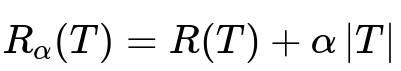
In this formula, T represents a candidate subtree (or the full tree after pruning), R(T) is the overall misclassification cost or impurity, alpha is a penalty factor for model complexity, and |T| denotes the number of terminal nodes in subtree T. The alpha term controls how aggressively we want to prune. A higher alpha leads to more pruning because it places a higher penalty on the size of the tree.

Pre-pruning can be faster in practice because we do not need to grow a very large tree before pruning. However, it risks stopping too soon and underfitting if the early stopping criteria are too strict. Post-pruning, though more computationally expensive, often yields a more accurate final model because it examines a fully grown tree and determines which parts truly help reduce error on validation data.

Practical Implementation Insights

In libraries like scikit-learn, there are parameters such as max_depth, min_samples_split, min_samples_leaf, and max_leaf_nodes that act as pre-pruning controls. These constraints effectively stop the tree from becoming overly large during training.

For post-pruning, one can use the parameter ccp_alpha (cost-complexity pruning alpha) in DecisionTreeClassifier or DecisionTreeRegressor. The usual workflow involves:

from sklearn.datasets import load_iris
from sklearn.model_selection import train_test_split
from sklearn.tree import DecisionTreeClassifier

X, y = load_iris(return_X_y=True)
X_train, X_test, y_train, y_test = train_test_split(X, y, random_state=42)

# Grow a fully expanded tree
clf_full = DecisionTreeClassifier(random_state=42)
clf_full.fit(X_train, y_train)

# Cost-complexity pruning path
path = clf_full.cost_complexity_pruning_path(X_train, y_train)
ccp_alphas = path.ccp_alphas  # array of alpha values to try

# For each alpha, train and evaluate
best_alpha = None
best_score = 0
for alpha_val in ccp_alphas:
    clf_pruned = DecisionTreeClassifier(random_state=42, ccp_alpha=alpha_val)
    clf_pruned.fit(X_train, y_train)
    score = clf_pruned.score(X_test, y_test)
    if score > best_score:
        best_score = score
        best_alpha = alpha_val

print("Best alpha:", best_alpha)
print("Best pruned-tree accuracy:", best_score)

This process is a typical example of post-pruning, where one grows a large tree first, then prunes it using different alpha values, and chooses the alpha that yields the best validation performance.

Potential Follow-up Questions

Why do we need pruning in decision trees?

Pruning is essential to mitigate the overfitting tendency of decision trees. An unrestricted decision tree can keep splitting until it reaches pure leaf nodes, capturing every small detail (and noise) in the training set. This can lead to excellent training accuracy but poor generalization. Pruning ensures that the model remains simpler, improving its performance on unseen data.

How does pre-pruning risk underfitting?

In pre-pruning, you stop the growth of a tree early based on some threshold, such as maximum depth or minimum samples required to split. If this threshold is set too conservatively, the model might not capture potentially important splits and relationships in the data, leading to underfitting. The tree fails to learn certain nuances because it was never allowed to expand into those regions of the feature space.

What are the benefits of post-pruning over pre-pruning?

By allowing the tree to grow fully, post-pruning can discover regions where splits genuinely reduce error. Then, using a separate metric like validation error or cost-complexity pruning, you selectively remove branches that do not generalize well. This procedure is more adaptive because it assesses splits in the context of the fully grown structure and does not prematurely discard potentially beneficial splits.

Could post-pruning become more expensive computationally?

Yes. Post-pruning typically requires the tree to be grown fully first, which can be computationally more intensive, especially if the dataset is large or if the tree ends up extremely deep. Moreover, the pruning step itself (which might involve searching over many possible subtrees or alpha values) further increases the computational burden compared to a strategy that stops early.

How do we choose alpha in cost-complexity pruning?

One approach is to use a validation set or cross-validation. You train the model with different values of alpha, measuring the performance on a validation set (or through cross-validation). The alpha that yields the best performance on validation data is selected. This avoids subjective tuning of alpha and ensures a systematic approach based on actual performance metrics.

When might pre-pruning be preferred in practice?

In time-critical applications or very large datasets, pre-pruning can be more practical because it reduces the training time by avoiding the full expansion of the tree. If you have strict computational constraints or the data is continuously updating in an online manner, pre-pruning might be a simpler and faster way to control tree size. It might not produce the absolute best model, but it can be effective when resources or time are limited.

Are there scenarios where pre-pruning might outperform post-pruning?

If your hyperparameters for pre-pruning are carefully tuned and the data distribution is well-understood, pre-pruning can sometimes produce a decent tree quickly. In highly noisy data, it might not be beneficial to let the tree grow to a large size only to prune it back later. In such cases, well-chosen pre-pruning rules might strike a good balance from the outset, though typically post-pruning is still considered more robust for optimal performance.

Could combining pre-pruning and post-pruning be beneficial?

Yes. Sometimes researchers apply mild pre-pruning (like a very large max_depth or a relatively small minimum samples split) to prevent the tree from becoming unwieldy or overfitting on outliers, and then they apply a post-pruning step. This ensures the training process is manageable while still allowing for a final model that is tuned through a pruning procedure.

How do you evaluate whether pruning was successful?

One standard approach is to compare performance metrics such as accuracy or F1 score on a validation set or through cross-validation before and after pruning. If the pruned model achieves similar or better performance with fewer leaves or reduced depth, then pruning has likely succeeded. Another indicator is improved performance on unseen data due to reduced overfitting.

Summary of Key Differences

Pre-pruning stops tree growth early, potentially saving computation time but risking missing useful splits. Post-pruning grows the tree fully and cuts it back later, usually resulting in a more accurate model but at a higher computational cost. Both approaches aim to prevent overfitting, each with its own trade-offs in model complexity, training efficiency, and performance on unseen data.