
ML Interview Q Series: How do Principal Component Analysis and Random Projection differ from each other?


📚 Browse the full ML Interview series here.
Comprehensive Explanation
Principal Component Analysis (PCA) is a classical dimensionality reduction technique that identifies directions (principal components) capturing maximum variance in the data. It is data-driven, as it must compute the covariance matrix or use the Singular Value Decomposition (SVD) of the original dataset.
Random Projection, on the other hand, is a method that uses a randomly generated transformation matrix to project the high-dimensional data into a lower-dimensional space. Rather than focusing on data covariance, the method’s effectiveness is often analyzed through concentration of measure and results like the Johnson-Lindenstrauss lemma, which state that pairwise distances are preserved with high probability.
Mathematical Underpinnings
PCA’s Core Idea
PCA finds a low-dimensional subspace by computing top eigenvectors of the covariance matrix. Suppose you have a dataset X with n samples and d features. Let C be its covariance matrix. PCA seeks to find directions (principal components) v that maximize data variance. One way to view the dimensionality reduction step is to project X onto these top k principal components.

Here, V_{k} contains the top k eigenvectors (principal components). Each vector in V_{k} is orthonormal, and X_{reduced} has dimensionality n by k. Parameters are:
X is the original n by d data matrix (each row is a data point).
V_{k} is a d by k matrix of the leading eigenvectors.
X_{reduced} is the transformed n by k data matrix.
Random Projection’s Core Idea
Random Projection draws a random matrix R (usually from some distribution such as a Gaussian or a sparse sign-based distribution) of size d by k and multiplies the original data points by this matrix to obtain a k-dimensional representation.
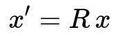
Where:
x is a d-dimensional data vector.
R is a d by k random matrix.
x' is the resultant k-dimensional projected vector.
Unlike PCA, this process does not rely on variance maximization or the data covariance structure. Instead, it leverages the idea that random linear projections approximately preserve pairwise distances in high-dimensional spaces with high probability.
Complexity and Scalability
PCA requires calculating the covariance matrix and then performing an eigen-decomposition or an SVD. For large datasets with very high dimensionality, this can be computationally expensive. While there are approximate or incremental variants of PCA, the classic method scales in complexity roughly with d^2 n (for computing the covariance and eigen-decomposition), depending on the implementation.
Random Projection typically has a simpler and faster implementation, since generating a random matrix and multiplying it by the data is more straightforward. It can be especially beneficial in extremely high-dimensional settings when a quick dimension reduction step is needed before using more advanced models.
Data Dependence vs. Data Independence
PCA directly leverages the data distribution. It discovers directions of largest variance, which can make the resulting reduced features more interpretable. The top principal components often correspond to meaningful patterns in the data.
Random Projection does not adapt to the data itself. It relies purely on a random matrix, which can be beneficial in privacy-sensitive contexts (no direct data imprint in the projection matrix) and in streaming or large-scale contexts (projection is easy to update if the distribution shifts).
Interpretability
PCA is widely used for data visualization and interpretation because each principal component can be associated with a combination of original features that reflects a certain direction of maximal variance. This can be examined to uncover underlying structure in the data.
Random Projection is more opaque. The resulting dimensions are random linear combinations of the original features. They have no direct interpretation in terms of the original feature set. Random Projection is typically used when interpretability is not the primary goal.
Preservation of Distances or Variances
PCA preserves directions of greatest variance, which is often beneficial for classification or regression tasks where variance in certain directions is crucial for predictive power.
Random Projection is analyzed based on the probability of preserving pairwise distances between points. With a sufficiently large projection dimension, the pairwise distances in the lower-dimensional space are close to those in the original space. However, it might not preserve data variance in a semantically “optimal” manner for a specific prediction task.
Practical Use Cases
PCA is often used in exploratory data analysis, data compression, and as a preprocessing step to remove correlated features before applying classification or regression methods.
Random Projection is used when data has extremely high dimensionality, or when speed and scalability are critical and one only needs distance preservation properties, not interpretability.
What if the Data Has Non-Linear Structure?
When the data is highly non-linear, linear methods like PCA might fail to capture important non-linear relationships. One might resort to kernel PCA or other manifold learning techniques. Random Projection still remains a linear transformation. If the data’s structure is strongly non-linear, both PCA and Random Projection may require additional steps or alternative strategies like kernel methods or deep autoencoders.
Are There Situations Where Random Projection Outperforms PCA?
There are scenarios with massive datasets, very high feature dimensionality, or strict time/memory constraints where random projection is much faster to compute than PCA. If the primary goal is to quickly reduce dimensionality to a manageable level before feeding data into a downstream algorithm (such as clustering or nearest-neighbor search), random projection can be an excellent choice. Although PCA might find a slightly better embedding with respect to variance or data representation, the computational cost can become prohibitive.
How Does the Johnson-Lindenstrauss Lemma Relate to Random Projection?
The Johnson-Lindenstrauss lemma states that for n points in a high-dimensional space, one can project them into a space of dimension proportional to log(n / epsilon^2) while approximately preserving the pairwise distances (within 1 ± epsilon). This provides a theoretical guarantee for the effectiveness of random projection in dimension reduction. Unlike PCA, which is not strictly bound by this lemma, random projection’s distance-preserving property is directly related to it.
Could PCA Lose Important Low-Variance Directions That Random Projection Might Keep?
PCA focuses on capturing the directions with the highest variance, which can inadvertently compress or lose potentially informative directions with smaller variance. In certain tasks, those low-variance directions might still contain relevant discriminative signals. Random projection does not prioritize variance; it randomly distributes the data into a new subspace, which may preserve aspects of low-variance directions. However, this is not guaranteed, and its success remains probabilistic.
How to Combine PCA and Random Projection in Practice?
Sometimes practitioners perform a hybrid approach. They may use PCA first to reduce extremely high dimension to a smaller intermediate dimension (ensuring they keep the main variability), and then apply a random projection to further compress the data if needed. This can strike a balance between preserving important data structure (from PCA) and achieving a large reduction in dimension (from random projection).
Are There Implementation Details to Be Aware Of?
In practice, you should consider:
Normalization of Data: PCA is often performed on mean-centered data, sometimes normalized by standard deviation. Random projection typically uses raw data or only simple scaling, depending on the application.
Random Matrix Distribution: For random projection, distributions like Gaussian or sparse sign-based distributions can be used. The choice can influence computational costs and performance.
Parameter Tuning: For PCA, one chooses k by examining eigenvalues or by specifying the fraction of variance to retain. For Random Projection, one chooses k based on the acceptable distortion of distances (often guided by the Johnson-Lindenstrauss lemma).
Overall, PCA and Random Projection each have specific advantages. PCA is typically more powerful for data interpretation and identifying dominant structure, while Random Projection is extremely fast, privacy-preserving, and theoretically well-founded for preserving distances in high-dimensional settings.