ML Interview Q Series: How do Region-Based CNN (R-CNN), Fast R-CNN, and Faster R-CNN differ from each other?

📚 Browse the full ML Interview series here.

Comprehensive Explanation

R-CNN, Fast R-CNN, and Faster R-CNN are all landmark approaches for object detection tasks in computer vision. Object detection requires identifying the correct position (bounding box) of each object within an image and classifying the object. The fundamental shift across these three methods lies in how they generate region proposals, how they share convolutional computations, and how they optimize for speed while maintaining accuracy.

R-CNN

Region-Based CNN (R-CNN) was one of the earliest deep learning-based methods to tackle object detection. The high-level idea is to generate region proposals through a separate module (like Selective Search) and then classify each proposed region using a CNN.

It first extracts about 2,000 region proposals that are likely to contain objects. Each region proposal is then cropped (or warped) to a fixed size and fed into a CNN (such as AlexNet in the original paper) for feature extraction. Finally, a classifier (like SVM) is used on top of those extracted features to classify each region, and a separate regression module refines the bounding box coordinates.

This approach was innovative but suffered from being computationally slow. Each region proposal had to be processed independently by the CNN. Storage also became an issue, because feature extraction for so many regions resulted in huge disk usage.

Fast R-CNN

Fast R-CNN introduced an important improvement that speeds up the process significantly. Instead of running the CNN on each region proposal independently, Fast R-CNN processes the entire input image once through a CNN to generate a convolutional feature map. Then, region proposals are projected onto the feature map. From those projected locations, a sub-region is extracted and pooled (through Region of Interest [RoI] Pooling) to produce a fixed-size feature. This feature is fed into fully connected layers and then into parallel heads for classification and bounding box regression.

This single forward pass is far more efficient because the shared convolutional feature map means that only one CNN pass is needed per image. The region-level computation is reduced to extracting and pooling from the shared feature map, which drastically speeds things up relative to R-CNN. However, Fast R-CNN still relies on an external algorithm like Selective Search for region proposal generation, which is often slow and not learnable end-to-end.

Faster R-CNN

Faster R-CNN took the next big step by introducing the Region Proposal Network (RPN), which makes region proposal generation part of the neural network itself. The RPN slides over the convolutional feature map (the same one shared by the main detection network), producing potential bounding boxes (called anchors) along with scores that reflect objectness. This approach replaces the external region proposal method (like Selective Search) with a fully convolutional, learnable network. Because RPN shares features with the detection network, it yields a significant boost in speed while maintaining or even increasing accuracy.

In Faster R-CNN, the shared backbone CNN produces feature maps, the RPN proposes regions, and the RoI pooling (or its improved variant RoI Align in later versions) extracts fixed-size features for each proposed region. The detection head finally classifies each region and refines the bounding boxes.

Key Architectural Differences

R-CNN uses an external region proposal algorithm and processes each region independently. This is computationally heavy since the CNN must be run for each of the thousands of region proposals.

Fast R-CNN only runs the main CNN once and performs region-wise computations by extracting RoIs from a shared feature map, significantly reducing the number of passes. Still, it depends on an external region proposal generator, which can be slow.

Faster R-CNN integrates region proposal generation into the network itself via the RPN, removing the need for an external proposal method and allowing end-to-end training. This is significantly faster and more accurate.

Core Mathematical Consideration: Bounding Box Regression

When any of these methods refine the coordinates of a bounding box, they often use a smooth L1 loss or a similar metric. A common bounding box regression loss can be expressed as follows:

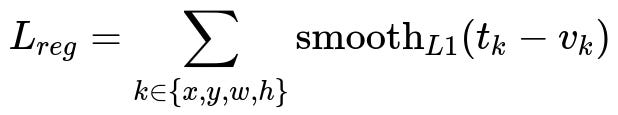
where t_k denotes the model’s predicted transformation for one of the bounding box parameters (x, y, width, and height), and v_k represents the ground truth transformation. The term smooth L1 is a function that behaves like L1 near 0 but is quadratic for smaller errors, stabilizing gradients. This bounding box regression step refines the coordinates proposed by either the external region proposal algorithm (R-CNN, Fast R-CNN) or the Region Proposal Network (Faster R-CNN).

Potential Follow-up Questions

How does RoI Pooling work, and why is it important?

RoI Pooling is designed to convert variable-sized region proposals into fixed-sized feature maps so that they can be fed into fully connected layers. It does this by spatially dividing the region of interest into a predefined grid (for example, 7x7), then applying max or average pooling within each grid cell. This step is important because fully connected layers require consistent input dimensions, and object proposals come in different shapes and sizes.

One subtlety to note is that RoI Pooling can cause misalignments due to quantization of boundaries. This was later improved by RoI Align, which removes the quantization step and samples more precisely to preserve spatial alignment, resulting in higher accuracy.

What role do anchor boxes play in Faster R-CNN?

In Faster R-CNN, the RPN uses anchors as predefined bounding boxes at each location on the feature map. For example, it might use anchors of different aspect ratios and scales at each pixel in the feature map. Each anchor is scored for objectness (does it contain an object or not?) and is also regressed to better fit the object if present. These anchors allow a single forward pass of the RPN to handle multiple scales and aspect ratios without separate region proposal methods.

A real-world pitfall is to choose a poor set of anchor scales or aspect ratios for your specific dataset. If they do not properly match the distribution of object sizes in your data, the proposals and final detection performance will suffer.

How do you train Faster R-CNN end-to-end if it has two different modules (RPN and final classifier)?

Faster R-CNN is typically trained in alternating phases or via joint training (multi-task learning). During alternating training, the RPN is trained to propose regions, then these proposals are used to train the detection head. One iteration of training updates the RPN, and another iteration updates the Fast R-CNN detection part, continually refining both. In practice, frameworks like PyTorch or TensorFlow can integrate these steps neatly so that the entire network can be trained in a more unified manner.

A common challenge is calibrating the losses of the RPN and the detection head. Hyperparameters like the balance weights for classification loss vs. bounding box regression loss can significantly affect performance.

Why did Fast R-CNN still rely on an external region proposal method even though it was faster than R-CNN?

Fast R-CNN shared convolutional computations, which improved speed over R-CNN. However, region proposals in Fast R-CNN were still generated by a selective search-like mechanism running on the input image. This external algorithm was not part of the deep network, so it could not benefit from GPU acceleration in a straightforward manner and was not learnable. Though classification and bounding box refinement were faster, generating proposals remained a bottleneck. That was the motivation behind Faster R-CNN, which replaced external proposals with a dedicated Region Proposal Network.

When would you still use R-CNN or Fast R-CNN instead of Faster R-CNN?

In most modern production or research scenarios, you would not revert to R-CNN or Fast R-CNN, because Faster R-CNN is generally more efficient and accurate. However, there are rare cases where older methods might be used for reference comparisons or for certain specialized tasks where external region proposals might produce better region candidates (for example, if you have a highly specialized domain where a custom region proposal generator is extremely effective).

Example of Using a Faster R-CNN Implementation in Python (PyTorch)

import torch
import torchvision
from torchvision.models.detection.faster_rcnn import FastRCNNPredictor

# Suppose we load a pretrained Faster R-CNN model from torchvision.
model = torchvision.models.detection.fasterrcnn_resnet50_fpn(pretrained=True)

# The pretrained model is for 91 classes (COCO). Let's say we have only 2 classes.
num_classes = 2

# Get the number of input features for the classifier
in_features = model.roi_heads.box_predictor.cls_score.in_features

# Replace the pre-trained head with a new one
model.roi_heads.box_predictor = FastRCNNPredictor(in_features, num_classes)

# Now 'model' is ready for training with two classes (background + object).
images = [torch.randn(3, 300, 300)]
labels = [{
    "boxes": torch.tensor([[50, 50, 200, 200]], dtype=torch.float32),
    "labels": torch.tensor([1], dtype=torch.int64)
}]
output = model(images, labels)  # returns the loss during training

This snippet shows how you can initialize a Faster R-CNN model in PyTorch, modify the classification head, and perform a forward pass with a dummy example. In practice, you would iterate over a dataset of images and bounding box annotations to train your model.

Could Faster R-CNN still be too slow for certain applications, and what are possible solutions?

Faster R-CNN is much faster than its predecessors, but it may still be slower than one-stage detectors (for example, YOLO or SSD) for certain real-time applications. If low latency is critical, you might consider these one-stage detectors. Alternatively, you can scale down the backbone or reduce input resolution to increase speed at the cost of some accuracy.

Using accelerators (GPUs, TPUs) or optimizing the network architecture (for example, using a MobileNet backbone for a lighter model) can also be effective strategies to achieve near real-time performance while leveraging the advantages of two-stage detection.

How do these models handle multiple objects of different scales?

Each of these architectures considers multiple scales either through external region proposals (R-CNN, Fast R-CNN) or through anchor boxes of different sizes (Faster R-CNN). Because each proposal or anchor can vary in scale and aspect ratio, the network learns to detect objects of various sizes. However, dataset diversity and correct hyperparameter tuning of anchor sizes are critical to ensure reliable detection across a wide range of object scales.

What are typical pitfalls when training or deploying these models?

Pitfalls include poorly tuned anchor settings in Faster R-CNN, improper non-maximum suppression thresholds leading to too many or too few detections, imbalanced training data across object classes, and insufficient GPU memory if the network is not sized properly. During deployment, ensuring consistent preprocessing, such as normalization and resizing, is essential. Another subtle point is the potential mismatch between training and inference image resolutions. If the training resolution differs significantly from deployment images, detection performance might degrade.

Below are additional follow-up questions

How do we handle class imbalance in multi-class detection scenarios with these frameworks?

Class imbalance is a common challenge because real-world datasets often contain many more examples of common classes compared to rare classes. This imbalance can cause the model to bias its predictions toward the majority class. In two-stage detectors like R-CNN variants, class imbalance can occur in two areas: the region proposals and the final classification head.

One approach is to use specialized sampling or weighting strategies. For instance, you can employ focal loss in the classification head to put more emphasis on hard or rare examples. Another method is oversampling the minority classes or undersampling the majority classes when creating mini-batches. A subtle pitfall is over-correcting the imbalance, which can result in higher false positive rates for minority classes. It is vital to strike a balance between making the model more sensitive to underrepresented classes and maintaining overall precision.

In practice, you might also implement class-aware sampling at the proposal level. For example, you can push the RPN to propose more regions for the rare classes if you have some prior knowledge (like typical location or size). However, such specialized solutions can be complex and might require domain-specific tuning.

What if the Region Proposal Network produces too many proposals or too few proposals?

The Region Proposal Network can output a large number of anchors, each with different scales and aspect ratios. If the RPN is producing too many proposals, the computational overhead for the RoI head could become large, leading to longer training and inference times. Moreover, too many proposals might increase the false positive rate if the post-processing step (like non-maximum suppression) is not calibrated properly.

On the other hand, if the RPN is too conservative and yields too few proposals, the final detection stage might miss objects entirely. This usually happens if the model has not been trained sufficiently or if the anchor design does not align well with the distribution of object sizes in your dataset.

A common solution is to tune the RPN’s scoring threshold and the non-maximum suppression threshold. You can also adjust anchor scales and aspect ratios. Monitoring the recall at this stage is critical; if the RPN recall is high (it rarely misses actual objects), but many proposals are still produced, you can prune them more aggressively. If the RPN recall is too low, you need to widen your anchor settings, adjust the training objective, or lower the threshold for proposed boxes.

How do these frameworks handle heavily overlapping bounding boxes, and how do you refine them during inference?

Heavily overlapping bounding boxes are common when multiple proposals converge on a single object, or when multiple objects are clustered. During inference, non-maximum suppression (NMS) is typically employed to prune redundant bounding boxes that significantly overlap. The detection head produces a classification confidence for each box, and NMS retains the box with the highest confidence among overlapping candidates.

However, NMS threshold tuning can be tricky. A higher threshold can leave many duplicate detections, while a lower threshold can inadvertently suppress nearby objects of the same or different classes. One subtle scenario is images with objects arranged closely (like people standing in a crowd). A too-aggressive NMS can mistakenly discard adjacent detections.

Bounding box refinement happens through regression. If two boxes overlap too much and have high classification confidence for the same class, the regression head might push them closer to a single, correctly localized bounding box. But sometimes, objects truly overlap in the real world, so you might need to refine the NMS threshold or apply a more sophisticated method like Soft-NMS, which penalizes lower confidence boxes less aggressively instead of discarding them.

How should you approach data augmentation for object detection with these models?

Data augmentation for object detection has additional considerations compared to image classification because you must transform not only the image but also the bounding box coordinates. Typical augmentations include scaling, random cropping, flipping, color jittering, and small rotations. Each augmentation must be applied consistently to the image and its bounding boxes.

One pitfall is cropping out objects partially or entirely, which can lead to incorrect bounding box labels if not handled properly. Some libraries provide utilities that ensure a minimum portion of the object remains in the frame. Another subtlety is random resizing. If your training pipeline drastically resizes images, small objects could become too small for the network to detect reliably. Balancing between enough variation (to improve generalization) and maintaining object visibility can be delicate.

Advanced augmentations like CutMix or Mosaic (popularized by YOLO) can also be adapted to R-CNN-based pipelines, but require careful bounding box management. Overly aggressive augmentation can degrade performance if it leads to unrealistic or contradictory bounding box placements.

What are some strategies to further reduce inference time or memory usage, especially in Faster R-CNN?

Even though Faster R-CNN is relatively fast among two-stage detectors, it can still be resource-intensive. Strategies for optimizing speed and memory usage include:

Using a lighter backbone. ResNet-50 consumes fewer resources than ResNet-101, for example, and MobileNet or EfficientNet variants can reduce compute needs further.

Decreasing input resolution. Reducing the image input size can speed up inference significantly, though at the cost of missing smaller objects.

Reducing the number of proposals from the RPN. You can lower the pre-NMS top-k or post-NMS top-k thresholds. If the object recall remains acceptable, this can provide a significant speed boost.

Quantization or pruning. Quantizing model weights (e.g., from 32-bit floats to 8-bit integers) and pruning less significant network connections can accelerate inference on compatible hardware.

Batch inference. If your hardware and the framework support it, batching multiple images at inference can sometimes be more efficient, though it requires enough memory and a batch-friendly setup.

A pitfall is to over-optimize for speed at the expense of accuracy, leading to poor detection outcomes. Each optimization should be measured not only in terms of speed gain but also in the context of mAP (mean Average Precision) or another relevant metric.

How do these methods handle partial occlusions and truncated objects?

Partial occlusion occurs frequently in real-world scenarios (e.g., vehicles behind each other, people standing in crowds). Because two-stage detectors rely on region proposals and subsequent classification, mild to moderate occlusions can sometimes be tolerated, especially if enough of the object is visible. The feature maps may still capture discriminative cues.

Severe occlusion or truncation can pose problems. If the RPN sees only a fragment of the object, it might score it low for objectness, especially during early training. One practical mitigation is to include occluded examples in the training set, so the network learns to identify partial shapes. Data augmentation can simulate occlusion by overlaying random shapes, although overdoing this could introduce noise.

A subtle pitfall arises when bounding boxes are consistently mislabeled for occluded objects, such as incorrectly including or excluding the occluding object in the bounding box. Ensuring accurate labeling in the presence of occlusion is crucial. Another strategy might involve higher-level context or instance segmentation to more accurately separate overlapping objects.

How can we incorporate multi-scale feature representations in Faster R-CNN to improve detection of both small and large objects?

Faster R-CNN typically uses a single feature map (from a specific backbone layer) for both the RPN and the detection head. However, large objects can dominate the receptive field, while small objects can be drowned out. To address this, researchers have proposed Feature Pyramid Networks (FPN), which produce multiple feature maps at different scales. Each scale can better capture objects of a corresponding size, resulting in improved performance on tiny and large objects alike.

An FPN-based Faster R-CNN architecture merges top-down and bottom-up layers of a backbone like ResNet, creating a pyramid of feature maps. The RPN then proposes regions from multiple levels, matching anchors to the most appropriate scale. This approach often yields higher detection accuracy across varied object sizes. A potential edge case is that if the dataset mostly contains objects of a single scale, the extra overhead from multi-scale feature maps might not yield a substantial benefit and can slow down training or inference slightly.

How do you handle domain shift when using R-CNN-based methods? For instance, training on synthetic images but deploying on real images.

Domain shift arises when the distribution of training data differs significantly from the target domain. R-CNN-based methods are prone to domain shift because small differences in texture, lighting, or shape distribution can cause lower detection accuracy in the real domain.

To mitigate this, domain adaptation or fine-tuning is typically employed. You can start with a model trained on synthetic data, then fine-tune on a small subset of real images, if available. Unsupervised domain adaptation methods might align feature representations from synthetic and real domains, reducing discrepancies in the backbone and detection heads. Another strategy is to employ generative adversarial networks (GANs) to make synthetic images appear more realistic, thereby narrowing the gap.

Pitfalls include overfitting to a small real-world dataset if you have limited labeled examples. Also, certain domain disparities (like completely different object styles or textures) might require a carefully designed adaptation algorithm beyond simple fine-tuning. Monitoring performance across both domains is important, especially if you still want the model to work well on synthetic data for some reason.