ML Interview Q Series: How do Support Vector Machines differ from Deep Learning methods?

📚 Browse the full ML Interview series here.

Comprehensive Explanation

Deep learning and Support Vector Machines (SVM) are two influential approaches in machine learning, differing primarily in how they represent data, learn complex patterns, and scale to large datasets. Deep learning is built around neural networks with multiple layers that automatically learn hierarchical feature representations, while SVM is a margin-based method that attempts to separate data using a linear or non-linear boundary with the maximum margin. Both can handle high-dimensional data, but the practical implementations, training methodologies, hardware requirements, and problem setups differ in significant ways.

Core Concept of SVM

The fundamental principle of SVM is finding a decision boundary that maximizes the margin between the separating hyperplane and the nearest data points (support vectors). This can be expressed with the following standard optimization objective for a linear SVM:

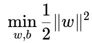
subject to y_i (w^T x_i + b) >= 1 for all training examples i.

Here, w represents the weight vector that defines the orientation of the hyperplane, b is a bias term that shifts the hyperplane, x_i are the training examples, and y_i are the labels (often +1 or -1 in binary classification). The constraints y_i (w^T x_i + b) >= 1 ensure that every example is on the correct side of the decision boundary, and maximizing the margin corresponds to minimizing the norm of w.

Core Concept of Deep Learning

A deep learning model, typically a deep neural network, consists of multiple stacked layers of neurons, each transforming its inputs through learned weights. In supervised learning, these networks often optimize a loss function (for example, cross-entropy loss for classification) through backpropagation. Instead of manually defining features, deep learning allows the network to learn representations of increasing complexity.

For a simple feed-forward neural network with L layers, the prediction for a single data point x can be viewed as repeated matrix multiplications and non-linear activations. Weights, biases, and activation functions all combine to learn intricate relationships. Deeper networks can extract higher-level abstract features.

Interpretability and Feature Engineering

One primary difference between SVM and deep learning is feature engineering. Traditional SVM applications often rely on manually engineered features or kernel functions to capture non-linearities in the data. Deep learning attempts to handle feature extraction internally, uncovering suitable representations for the task at hand if provided with sufficient data.

SVM can be more straightforward to interpret in terms of support vectors and margins. Deep neural networks, though, are generally seen as black-box models with weights and connections that are less interpretable. However, techniques like Layer-wise Relevance Propagation or saliency maps can be employed to glean insights from deep networks.

Computational Complexity and Scalability

Deep learning generally scales better with large datasets and can leverage GPU acceleration to train massive models with millions or billions of parameters. Large dataset availability is often considered a prerequisite for deep networks to outperform other methods.

SVM, especially with non-linear kernels, can become computationally expensive with increasing data size, because training complexity often grows more than linearly with the number of samples. In practical scenarios with large-scale data, one often resorts to approximate or linear SVM variants, or moves to deep learning solutions.

Practical Usage and Real-World Applications

SVM is typically employed in smaller or medium-sized datasets, where the dimensionality is high, but the number of samples is not extremely large. It can also work well in settings where interpretability of the margin or support vectors is important.

Deep learning has gained popularity in domains such as computer vision, natural language processing, and speech recognition, where large-scale datasets are abundant and complex feature hierarchies are necessary. Neural networks have proven to be highly effective once enough data and computational resources are available.

Example Code Snippet for SVM

from sklearn import svm
from sklearn.model_selection import train_test_split
from sklearn.datasets import make_classification
from sklearn.metrics import accuracy_score

# Generate a synthetic dataset
X, y = make_classification(n_samples=1000, n_features=20, random_state=42)

# Split into training and test sets
X_train, X_test, y_train, y_test = train_test_split(X, y, test_size=0.3, random_state=42)

# Create and fit an SVM model
model = svm.SVC(kernel='linear')
model.fit(X_train, y_train)

# Make predictions
predictions = model.predict(X_test)
print("SVM Accuracy:", accuracy_score(y_test, predictions))

Example Code Snippet for a Simple Deep Neural Network

import torch
import torch.nn as nn
import torch.optim as optim
from torch.utils.data import DataLoader, TensorDataset

# Generate random data (features and labels)
X = torch.randn(1000, 20)
y = torch.randint(0, 2, (1000,))

# Create a Dataset and DataLoader
dataset = TensorDataset(X, y)
loader = DataLoader(dataset, batch_size=32, shuffle=True)

# Define a simple fully-connected model
class SimpleNN(nn.Module):
    def __init__(self, input_dim, hidden_dim, num_classes):
        super(SimpleNN, self).__init__()
        self.fc1 = nn.Linear(input_dim, hidden_dim)
        self.relu = nn.ReLU()
        self.fc2 = nn.Linear(hidden_dim, num_classes)

    def forward(self, x):
        out = self.fc1(x)
        out = self.relu(out)
        out = self.fc2(out)
        return out

model = SimpleNN(input_dim=20, hidden_dim=50, num_classes=2)
criterion = nn.CrossEntropyLoss()
optimizer = optim.Adam(model.parameters(), lr=0.001)

# Train the network
for epoch in range(5):
    for batch_X, batch_y in loader:
        optimizer.zero_grad()
        outputs = model(batch_X)
        loss = criterion(outputs, batch_y)
        loss.backward()
        optimizer.step()

# The trained model can now be used for predictions

What are potential pitfalls when choosing between SVM and Deep Learning?

When making a choice, one pitfall is overestimating the ability of deep neural networks on very small datasets. With inadequate data, a deep model may overfit, yielding suboptimal results compared to a well-tuned SVM. Another pitfall is assuming that SVMs cannot work well at scale; in practice, linear SVMs or approximate kernel methods can handle relatively large datasets. Overlooking the significant resource requirements (e.g., GPUs) and hyperparameter tuning complexity for deep models can also pose problems if the infrastructure is insufficient.

How do hyperparameters differ for SVM and Deep Neural Networks?

In SVM, the main hyperparameters often revolve around the choice of kernel (e.g., linear, RBF), the regularization parameter C, and any kernel-specific parameters such as gamma for the RBF kernel. While these can be tuned with techniques like grid search, the parameter space is relatively small compared to large neural networks.

Deep networks have hyperparameters related to network architecture (number of layers, number of neurons per layer, types of layers, activation functions, dropout rate) and optimization (learning rate, batch size, momentum, weight decay, scheduler strategies). This increases the complexity of tuning because each hyperparameter can profoundly affect the learning process.

How might transfer learning change the comparison?

Transfer learning enables a deep neural network to leverage knowledge from a model pre-trained on a large corpus (e.g., large image datasets) and adapt it to a smaller target dataset. This typically offers a performance advantage over SVM for tasks like image recognition or text classification, even with fewer training samples, because the network already possesses relevant feature representations. In contrast, SVM typically does not benefit from such an extensive notion of “transfer” unless the features are carefully engineered or extracted from another model.

When is interpretability more straightforward in SVM than in Deep Learning?

SVM interpretability is often more direct because you can look at the support vectors (examples that define the decision boundary) and coefficients in the linear case. For the linear kernel, the weight vector w can reveal which features contribute most strongly to the classification boundary. Deep learning, with thousands or millions of parameters, does not grant such a straightforward interpretation without specialized methods like Grad-CAM, Integrated Gradients, or other model interpretability techniques.

What is the role of kernel tricks in SVM compared to representation learning in Deep Networks?

Kernel tricks allow SVMs to implicitly map input data into high-dimensional feature spaces without explicitly computing coordinates in that space. This enables flexible decision boundaries capable of handling complex patterns. However, the kernel’s functional form must be fixed in advance and carefully chosen.

Deep neural networks learn feature transformations directly from data across multiple layers. Instead of selecting kernels, the network updates its weights via backpropagation to capture complex, task-specific transformations. This automatic feature learning is a key advantage when large datasets are available, though it can lead to significant computational overhead and complexity compared to classic SVM solutions.

Below are additional follow-up questions

When might SVM outperform a Deep Neural Network in practice?

SVM can excel when the dataset is not large, but the features are high-dimensional and discriminative. In scenarios where a well-chosen kernel function can capture the complexity of the data, SVM often provides strong results without requiring massive amounts of labeled examples. This can happen in specialized domains where collecting large datasets is impractical (for example, certain biological or medical data).

One subtle pitfall is overlooking that a deep network might overfit if the dataset is too small. A carefully tuned SVM, coupled with proper regularization and feature engineering, might achieve better generalization. Another subtle issue is that deep networks often need well-initialized weights or advanced optimizers; if these are not configured properly, an SVM solution might converge to a more robust decision boundary faster and with fewer resources.

How does memory usage compare for SVM versus Deep Neural Networks?

Deep networks typically store a large number of parameters, especially in layers that include many neurons or filters (as in CNNs). This can lead to a significant memory footprint for both training and inference. On the other hand, an SVM’s memory footprint is tied to storing the support vectors and associated parameters. For a linear SVM, this can be relatively small if the number of features is not excessively large. However, non-linear SVMs with certain kernels may need to store a considerable portion of the training set as support vectors, leading to memory usage that grows with dataset size.

In real-world deployments, if a model must run on edge devices with limited RAM, a compact SVM might be more appropriate if it is sufficiently accurate. A large deep network would be unsuitable if it exceeds memory constraints. A subtle pitfall is ignoring that certain hardware (e.g., embedded systems) cannot support the large memory footprint needed for deep network inference.

How do their training times differ, and what factors influence those times?

Deep neural networks can require a substantial number of epochs over large datasets, with each epoch potentially taking significant time. GPU acceleration can mitigate this, but setting up a distributed or GPU-accelerated environment is non-trivial. Factors like model depth, layer size, and optimization technique also heavily influence training durations.

For SVM, linear versions train quite quickly on moderate-to-large datasets due to efficient solvers (e.g., stochastic gradient-based or coordinate descent methods). However, using sophisticated kernels can lead to training times that grow super-linearly with the dataset size. Additionally, selecting hyperparameters like C (the regularization parameter) and gamma for RBF kernels can be time-consuming if done exhaustively.

A pitfall is ignoring the precomputation step for some kernels: while this might speed up repeated training, it requires memory and overhead. Similarly, one can underestimate the time needed to tune neural network hyperparameters (architecture, learning rates, dropout, etc.). In some cases, automated hyperparameter search can become extremely time-intensive.

How do data preprocessing strategies differ between SVM and Deep Neural Networks?

Traditional SVM approaches often rely on careful feature engineering and possibly kernel selection. This might include normalization, feature scaling, dimensionality reduction (like PCA), or specialized transformations. The choice of kernel function effectively replaces part of the deep feature-learning process.

Deep neural networks typically learn representations directly from raw or minimally preprocessed data (e.g., raw pixels for images). While normalizing input features (for example, standardizing each feature to zero mean and unit variance) can still help, deep networks can discover sophisticated features if given enough labeled data. Data augmentation is also common in deep learning to artificially expand the training set (random crops, flips in images, etc.), which is less typical with SVM unless the augmentation translates neatly into the feature space.

A subtle pitfall in real-world scenarios: SVM might require rigorous domain-specific feature crafting, which is error-prone. In contrast, deep networks reduce the need for manual feature engineering but can fail if the domain data is not adequately represented or if the raw signals are too noisy.

In what ways do class imbalance issues affect SVM vs. Deep Learning models?

Class imbalance can pose challenges in both methods. For SVM, if one class is heavily represented among the support vectors, the boundary might shift and underrepresent minority classes. Techniques such as adjusting class weights (e.g., setting a higher penalty for misclassifying minority samples) or oversampling can mitigate this.

For deep learning, imbalanced data can also skew the loss toward predicting the dominant class. Data-level strategies like oversampling the minority class, undersampling the majority class, or using focal loss can help. Network-based strategies, such as adding cost-sensitive terms or employing novel layer designs, also address imbalance.

A hidden pitfall is assuming that large neural networks alone “solve” imbalance without additional measures. Deep networks can still converge to trivial predictions that favor the majority class if not carefully monitored. Similarly, SVMs are often believed to handle small datasets gracefully, but extremely skewed distributions can still degrade performance if no balancing methods are used.

Can outlier or noisy data impact SVM and Deep Neural Networks differently?

In SVM, outliers can become support vectors if they lie near or on the margin boundaries, affecting the decision surface disproportionately. The slack variable in soft-margin SVM partially handles outliers, but extreme outliers can still cause margin shrinkage.

In deep networks, outliers might lead to noisy gradient signals. Because of batch-based training, small portions of extreme values could push gradient updates in erratic directions. Regularization techniques (dropout, weight decay) help, but large amounts of noise in the data can hamper convergence or degrade model performance.

A real-world pitfall is failing to detect mislabeled data when training either model. Both methods can be misled by incorrect labels that function like outliers. SVM might overfit on such mislabeled points, and a deep network could embed these wrong labels into deeply learned representations. Proper data cleaning or robust training techniques (like robust loss functions) are essential to mitigate this issue.

How does online or incremental learning differ for SVM and Deep Neural Networks?

Online or incremental learning implies updating the model as new data arrives, without needing the entire dataset in memory. For linear SVM, stochastic gradient-based or online coordinate descent algorithms exist that can incrementally update the model parameters. Non-linear SVM with kernels is more challenging for online learning, since storing and managing kernel expansions incrementally can be computationally intensive.

Deep neural networks can also perform online learning by updating weights with each new batch. However, large networks might forget earlier learned knowledge if not carefully managed (the catastrophic forgetting problem). Methods like experience replay or specific architecture designs (e.g., elastic weight consolidation) can mitigate catastrophic forgetting, but they add complexity.

A hidden pitfall is ignoring the stability-plasticity trade-off in online learning for deep networks. Too much plasticity leads to forgetting old concepts; too much rigidity leads to poor adaptation to new data. SVM might handle incremental changes more predictably if using simpler variants, but again, kernel-based methods can become unwieldy.

Does interpretability differ for boundary decisions in multi-class settings?

In multi-class problems, SVM often uses one-vs-one or one-vs-rest schemes, where multiple binary classifiers are combined. Interpreting the final decision can be trickier because multiple binary SVMs vote or aggregate margins. While each binary decision boundary can still be inspected, the combined multi-class boundary can be less transparent.

Deep neural networks for multi-class classification typically output a probability distribution over classes via a softmax layer. While seeing which class has the highest predicted probability is straightforward, understanding which internal features led to that final decision is more complex. Techniques such as class activation maps or gradient-based attribution can shed light, but they require additional steps.

A subtle pitfall is believing that multi-class expansions of SVM remain as interpretable as the binary case. With many classes, the number of pairwise boundaries grows quickly, and analyzing them becomes cumbersome. In deep networks, interpretability relies heavily on specialized visualization or attribution methods, which can be non-trivial to implement and might offer partial rather than full transparency.