
ML Interview Q Series: How do we typically quantify the concept of information when constructing a decision tree?

📚 Browse the full ML Interview series here.
Comprehensive Explanation
Decision trees commonly use measures of impurity or uncertainty to quantify the information at each split. The higher the impurity (or uncertainty) in the target variable distribution, the more “mixed” or unpredictable the samples in that node. When a split reduces that impurity, we say we have gained information. Although there are multiple ways to measure impurity, the most classic approach is to use Entropy and Information Gain.
Entropy is a fundamental concept from information theory. In a decision tree context, it captures how unbalanced (or unpredictable) the class distribution is at a node. A pure node (e.g., 100% samples of one class) has zero entropy. A perfectly uniform node (e.g., 50% samples from two classes) has maximum entropy.
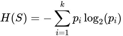
Below is the key formula for Entropy of a set S with k distinct classes. p_i is the probability (or relative frequency) of class i in set S.
where:
k is the total number of classes in the current node.
p_i is the fraction of samples belonging to class i in that node.
The log base 2 expresses the uncertainty in bits. If p_i is 0 for some class, then the term p_i log2(p_i) is conventionally treated as 0 because that class does not appear in the node.
Information Gain measures the reduction in entropy from splitting a node S using an attribute A. Let Values(A) be the distinct values or partitions of attribute A (for discrete features, those might be categories; for continuous features, typically thresholds). If S_v is the subset of samples of S where A has value v, then the information gain is:

where:
IG(S, A) is the information gain obtained by splitting set S based on attribute A.
H(S) is the entropy of the original set S.
H(S_v) is the entropy of the subset S_v.
|S_v|/|S| is the fraction of samples that end up in subset S_v after applying the split.
A larger value of information gain indicates a better (i.e., more “informative”) attribute for splitting because it reduces more entropy. In practice, the decision tree algorithm evaluates each candidate attribute (or threshold) and picks the one that yields the highest information gain at each node.
Another frequently used criterion is the Gini Index. It’s defined in many references as sum over all classes of p_i * (1 - p_i). The Gini index provides a similar sense of impurity, typically ranging between 0 (pure) and up to a maximum for a uniform distribution. Although sometimes Gini is explained in theoretical terms differently from entropy, both measure impurity, and in many practical scenarios, they often lead to very similar resulting trees.
Decision trees build top-down by recursively splitting the dataset to maximize information gain (or reduce Gini). Splitting continues until further partitions do not lead to any appreciable gain, or until other stopping criteria are met (like max depth or min samples per leaf). Pruning techniques are applied later if necessary, to avoid overfitting and to ensure generalization.
Below is a simple Python snippet illustrating how you might compute entropy and information gain for a single split. This is mostly for conceptual clarity:
import math
from collections import Counter

def entropy(samples):
    label_counts = Counter(samples)
    total = len(samples)
    result = 0.0
    for label, count in label_counts.items():
        p = count / total
        result -= p * math.log2(p)
    return result

def information_gain(parent_samples, subsets):
    # subsets is a list of sublists, each containing samples for one branch of the split
    parent_entropy = entropy(parent_samples)
    total = len(parent_samples)
    weighted_sum = 0.0
    for subset in subsets:
        weighted_sum += (len(subset) / total) * entropy(subset)
    return parent_entropy - weighted_sum

# Example usage
labels = ['cat','cat','dog','dog','dog','lion']
subsets = [
    ['cat','cat','dog'],
    ['dog','lion']
]
print("Entropy of parent:", entropy(labels))
print("Information Gain:", information_gain(labels, subsets))
These calculations demonstrate the essence of how decision trees quantify “information.” By measuring the decrease in entropy, we determine how much more certain we become about the class labels after splitting on a feature.
Could you elaborate on the difference between Entropy and Gini Index?
Both entropy and the Gini index track how impure a node is. Entropy is grounded in information theory and uses the formula involving p_i log2(p_i), whereas Gini is more of a measure of statistical dispersion, summing p_i * (1 - p_i). Entropy grows faster near the extremes of distribution, whereas the Gini index is simpler to compute. Practically, the choice between them seldom leads to vastly different performance. Entropy might provide slightly more nuanced splits in certain distributions, while Gini often has a simpler computational form and is sometimes faster in large-scale applications.
Why might someone choose Gini over Entropy in practice?
Gini index computations can be marginally faster because it avoids the log operation. Especially if you have a large dataset and are iterating over many candidate splits, that small difference can add up. Furthermore, some find Gini index to be more straightforward to interpret as a measure of misclassification potential. However, the performance difference is typically minor, and the choice often depends on convention or simply using the default setting of a particular library.
If decision trees measure information via Information Gain, how do we handle continuous features?
For a continuous feature, a common approach is to consider possible thresholds that split the data into “less than threshold” vs. “greater than or equal to threshold.” The algorithm searches over candidate thresholds (often found by sorting the feature values and evaluating splits between distinct values). Each threshold yields a split, and the algorithm computes the information gain for each potential split. The threshold with the highest information gain is chosen.
How do we address overfitting when using information-based splits?
If we keep splitting nodes until they are entirely pure, a decision tree can become very deep and overfit the data. We address this by imposing constraints or by pruning:
Early stopping: Limit tree depth, require a minimum number of samples per node, or impose a minimum information gain threshold for splitting.
Pruning: Grow the full tree, then prune back sub-branches that offer negligible improvement on a validation set or that fail statistical significance tests.
When might information gain be misleading?
Information gain can sometimes favor attributes with many distinct values, even if they do not generalize well. For example, an ID-like attribute that is unique for nearly every sample might yield a high apparent information gain by splitting into many subgroups of size 1, but that split is obviously not useful for generalization. In practice, many implementations use Gain Ratio (which normalizes by the split entropy) or rely on randomization/regularization methods to handle such cases.
Are there any other metrics beyond Entropy or Gini Index for measuring information?
Yes. Some variations include:
Misclassification Error: The fraction of incorrectly labeled samples in a node if one chooses the majority class. This measure is less sensitive than entropy or Gini to changes in node purity, so it is less popular for creating splits, though it can be useful for pruning.
Gain Ratio: An extension of information gain that penalizes splitting into many partitions, often used in C4.5 trees.
Variance Reduction: Used sometimes in regression trees, measuring the decrease in variance of the target value.
All these criteria are ways to quantify how “informative” or “valuable” a particular split might be in reducing uncertainty about the target variable.
Could you show a scenario where different impurity metrics lead to different splits?
Yes, though in many real datasets, Entropy and Gini produce very similar splits. Occasionally, a feature might yield the same information gain but a slightly different Gini gain, creating a different tie-break. The choice can change the exact split threshold or the shape of the tree. Typically, these differences are more about subtle local decisions than drastic final model differences. Some specialized distributions might be sensitive enough that these small differences become more pronounced, but that is not very common in practice.
How do we practically compute or apply these measures in libraries like scikit-learn or XGBoost?
In scikit-learn, you can specify a criterion parameter in DecisionTreeClassifier (e.g., criterion="entropy" or criterion="gini"). The library internally handles the computations of entropy or Gini. XGBoost uses a gradient-based approach for building trees but is still conceptually similar—aiming to find splits that maximize an objective function related to impurity reduction in the gradient sense. In both frameworks, you typically do not manually compute the splits. You only choose the criterion or objective, and the library automates the process.
All these details reflect the underlying principle of measuring how much a split reduces uncertainty or impurity. This idea is central to why decision trees are intuitive: each question you ask (i.e., each split) should reduce the overall confusion about the final class label or the numeric target value.