
ML Interview Q Series: How do you transform a Skewed distribution into a Normal distribution?


📚 Browse the full ML Interview series here.
Comprehensive Explanation
A skewed distribution means the data are not symmetrically distributed around the mean. In many machine learning or statistical tasks, it is often desirable to have a distribution that appears closer to a normal (Gaussian) shape. There are multiple approaches to achieve this transformation.
Using Power Transformations
One of the most common ways to reduce skew is by applying power transformations. The logic is to apply a function that systematically modifies every data point in a way that counteracts the skew. For right-skewed data, it is typical to apply transformations such as a logarithmic transform, square root transform, or Box-Cox. For left-skewed distributions, one might apply an appropriate power or shift the data before applying transformations.
The Box-Cox transformation is a well-known power transformation. In principle, it finds an optimal exponent lambda to transform the data so that it becomes more Gaussian. A generalized form of the Box-Cox transform can be written as follows.
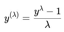
Below this formula, it is customary to define that if lambda=0, the transformation is the natural log of y. In this expression, y is the original data point, lambda is the transformation parameter (found by maximizing a certain likelihood measure that attempts to normalize the data), and y^(lambda) is the transformed data point.
If you encounter negative or zero values in your data, the Box-Cox transform might not be directly suitable without shifting the data by a positive constant first. Alternatively, you can use Yeo-Johnson transformations, which can handle zero or negative values more gracefully.
Using Logarithmic Transformation
When data is strictly positive and heavily right-skewed, you might consider a simple log transform. You replace each data point y with log(y). This helps in compressing large values and expanding smaller values, thereby bringing the distribution closer to normal if the original skew is caused by large outliers on the right side. For left-skewed data, a reflection might be done prior to applying the log.
Implementation in Python
Below is a brief example showing how to apply a Box-Cox transformation using scikit-learn:
import numpy as np
from sklearn.preprocessing import PowerTransformer

# Suppose data is a 1D NumPy array
data = np.array([10, 12, 15, 20, 35, 40, 100, 200]).astype(float)

# The PowerTransformer with method='box-cox' can handle strictly positive values
pt = PowerTransformer(method='box-cox')
data_transformed = pt.fit_transform(data.reshape(-1,1))

print("Original Data:", data)
print("Transformed Data:", data_transformed.flatten())
You would typically check the distribution of data_transformed (for instance using a histogram or a Q-Q plot) to verify that it is closer to a normal shape.
Potential Caveats
Not all distributions can be made perfectly normal merely by these transformations. For instance, if the data is multimodal or has a very long tail, standard power transformations may not suffice. In these cases, advanced transformations or distribution-specific techniques might be required.
Follow-Up Questions
Can you explain how the parameter lambda is found in the Box-Cox transformation?
The parameter lambda is typically chosen to maximize the log-likelihood of the transformed data under the assumption that the result follows a normal distribution with constant variance. The transformation tries different lambda values and uses an optimization procedure (like a grid search or a derivative-based method) to find the lambda that best normalizes the data.
It is important to remember that the Box-Cox transform requires all data points to be strictly positive. If any data value is zero or negative, a positive shift may be applied to all points prior to the transform.
What happens if lambda is found to be zero?
When lambda approaches zero, the Box-Cox transformation reduces to a natural logarithm transform. Mathematically, if lambda=0, the expression y^(lambda) can be interpreted as log(y), which is one reason Box-Cox transformations and log transformations are related. Practically, the software implementation often checks if lambda is near zero and simply applies the log function.
How would you handle negative or zero values in your data?
Box-Cox transformations cannot be directly applied to data containing zero or negative values. A common workaround is to shift the entire dataset by a positive constant, ensuring all values become strictly positive. Another approach is to use Yeo-Johnson transformations, which were designed to handle zero or negative values without a preliminary shift.
When should one consider applying a power transformation to a feature in a machine learning pipeline?
It is most beneficial when the feature’s skew significantly hampers model performance or when the model you are using makes strong distributional assumptions. Some linear-based algorithms may benefit from normally distributed error terms, making transformations helpful in stabilizing variance and making the model’s errors more Gaussian. Additionally, transformations can reduce the impact of outliers.
Could there be any drawbacks to applying these transformations?
Applying power transformations can complicate model interpretation because your features become transformed. For example, if you transform a target variable using a log transform, the model’s outputs are now in log-scale and must be exponentiated to interpret them in the original scale. Moreover, over-zealous transformation of every skewed feature can add unnecessary complexity if the model might learn the skew without transformation, as can happen with certain tree-based or neural network models that are robust to non-Gaussian distributions.
Below are additional follow-up questions
How can you determine if a transformation has actually improved the normality of your data?
A common way is to analyze diagnostic plots or statistical metrics of normality before and after the transformation. For instance, you can:
Plot histograms of the pre- and post-transformed data to visually assess skew reduction or changes in the distribution’s shape.
Generate Q-Q (Quantile-Quantile) plots: Ideally, points in a Q-Q plot should lie close to the reference diagonal if the distribution is normal. Deviations from this diagonal indicate departures from normality.
Use statistical tests such as the Shapiro–Wilk test or Kolmogorov–Smirnov test. They evaluate the likelihood that the data come from a normally distributed population. After transformation, you can compare p-values or test statistics to gauge improvement.
A potential pitfall is over-reliance on any single diagnostic. For example, Q-Q plots can fail to highlight issues if you have very large datasets (where even minor deviations might appear significant) or if you only rely on one type of normality test. In real-world scenarios, it’s prudent to combine visual methods, statistical tests, and domain knowledge.
What considerations apply when you have a mix of continuous and discrete variables in your dataset?
If some features are skewed continuous variables (like incomes or house prices) and others are categorical, you have to decide which features merit transformation. Typically, transformations are for continuous variables, but:
Categorical variables with many levels can sometimes be encoded in ways that inadvertently mimic continuous data. Careful one-hot or target encoding could be a better approach than forcing a power transform on a nominal feature.
When you have discrete count data (e.g., number of events) that exhibit skew, you might try transformations such as a log transform, but you need to be wary of zero or near-zero counts which could lead to undefined or highly distorted values. A small offset (e.g., log(x+1)) can mitigate that.
Skew in categorical distributions (like one category being extremely frequent compared to others) is not directly addressable by power transformations. Instead, you might look at re-balancing strategies or binning categories.
A subtle issue is that applying transformations to a subset of features while leaving others unaltered can complicate interpretability. Consistency in your pipeline is key, and you should document any transformations meticulously.
What if you have strong outliers that remain even after transformations?
Although power transformations like log or Box-Cox can reduce the impact of high outliers, extreme data points might still exist. You should investigate why those outliers occur:
They may be legitimate observations in a “heavy-tailed” domain (like financial transactions where rare but massive values are real).
They may be data entry errors or anomalies that should be treated or removed.
If the outliers are genuine but severely distort your distribution, you may need robust techniques beyond standard transformations. Methods such as robust scaling (which uses medians and interquartile ranges) or trimming/extreme value analysis might be necessary. A pitfall here is that indiscriminate outlier removal can lead to biased results, especially if those large values are systematically related to an important factor in the problem.
When might you consider splitting the dataset instead of applying a global transformation?
Sometimes, a dataset can be a mixture of multiple subpopulations that each have a different distribution. For instance, if you have a dataset of incomes from vastly different regions or groups, the combined distribution might appear heavily skewed and bimodal or multimodal.
In these cases, forcing a single transformation (like Box-Cox) on the entire dataset may not fix the fundamental issue that you really have multiple distributions in one place. Instead, you might:
Split the dataset into subgroups based on known criteria (e.g., region, demographic, or business unit).
Fit separate models or apply separate transformations for each subgroup.
Recombine the predictions or analysis afterward as needed.
A potential pitfall is overfitting or data leakage when splitting without a strong theoretical or domain-based reason. Splitting also reduces sample size in each subgroup, so you have to ensure each subgroup is sufficiently large to train reliable models or perform robust transformations.
How can transformations fit into cross-validation or pipeline processing without leaking information?
Data leakage occurs if you fit a transform using the entire dataset and then use that transform on your test or validation data. This artificially inflates performance measures since the transform parameters (like Box-Cox lambda) are influenced by all data points, including those in the test fold.
To avoid this, you should integrate transformations into a pipeline:
Within each cross-validation fold, fit the transformer (e.g., Box-Cox, log, Yeo-Johnson) only on the training portion of that fold.
Apply the learned transformation to the validation subset in that fold.
Evaluate your model on the transformed validation data.
By ensuring the transformation step is part of the pipeline that runs inside cross-validation, you avoid leaking transformation parameters. A pitfall is forgetting to include the inverse transform for post-processing steps if you need predictions back in the original scale (particularly for regression tasks).
Under what circumstances might power transformations fail to make the data normal?
Power transformations, including Box-Cox or Yeo-Johnson, assume that the data can be approximated by applying a monotonic function. If the true distribution is highly irregular, multimodal, or constrained by domain-specific phenomena, a simple exponent-based transform might not be sufficient. Examples include:
A distribution with structural zeros (e.g., data on drug usage where many individuals might have zero usage).
Strongly multimodal data representing different underlying processes.
Highly discrete counts that do not easily map to continuous-like distributions.
In such cases, a single power parameter cannot capture the necessary shape changes to force normality. You might opt for more specialized transformations or distribution-specific modeling (e.g., zero-inflated Poisson models in count data). One pitfall is assuming any data can be “fixed” by the right exponent, leading you down a dead end if the distribution is fundamentally not amenable to being reshaped into normal.
Do transformations always benefit complex models such as neural networks or gradient boosting machines?
Many tree-based and neural network models can inherently learn complex relationships and are relatively robust to skewness compared to linear models. In fact, tree-based methods split data along any chosen feature values, making the shape of the distribution less critical to performance.
However, transformations can sometimes still help:
It can stabilize variance, making optimization (particularly in neural networks) more stable and gradient updates more balanced.
It can mitigate the impact of extreme outliers on model training.
In certain scenarios, particularly where interpretability is crucial, transformations might complicate the interpretation of feature importances or weights. A potential pitfall is applying transformations by default, even when your model can handle skew well. It might introduce additional hyperparameters (like the lambda in Box-Cox) and complexity, with minimal performance gain.
What if you only transform the target variable in a regression problem?
Transforming the target variable (e.g., applying a log transform to predict log(y) instead of y) can be beneficial if the target is highly skewed or positive-only, such as sales or prices. By doing so:
You can reduce the influence of very large target values.
The model’s residuals might become more homoscedastic and closer to normal.
Interpreting the model’s predictions in the original scale requires applying the inverse transformation (e.g., exponentiating the log-predictions). Any metrics that rely on raw prediction errors (like RMSE in the original space) also require reversing the transformation to interpret them properly. A subtlety is that transforming the target modifies the loss function. For example, an MSE on log(y) is effectively a relative error measure. You need to be aware of the trade-off between modeling in the transformed space and what your evaluation metric requires.