
ML Interview Q Series: How do you handle 20% missing square footage in 100,000 Seattle home sales for price prediction?

📚 Browse the full ML Interview series here.
Comprehensive Explanation
Nature of the Missing Data
In a housing dataset, missing entries—especially in crucial fields like square footage—can drastically influence our model’s performance. Missingness can occur due to a range of factors: data collection errors, older listings with incomplete records, or purposeful omission by sellers. Before deciding on a method to handle the absent square footage, it is vital to investigate why these values are missing. If the data are Missing Completely at Random (MCAR), simpler strategies like mean or median imputation might suffice. If the data are Missing at Random (MAR) or Missing Not at Random (MNAR), more advanced techniques that leverage correlated features are typically needed.
Potential Strategies for Handling the Missing Data
Strategy A: Dropping Rows
One simple approach is to discard the entries lacking square footage. However, since 20% of the data is missing, dropping them outright could:
Substantially reduce the volume of training data.
Introduce bias if the missingness is not random.
Because 20% is a sizable fraction, this approach is typically not recommended unless further investigation shows that the missing records do not contribute meaningful patterns, or the dataset is still abundant enough to maintain reliable model performance.
Strategy B: Simple Statistical Imputation
A common approach is to fill missing square footage values with a single statistic:
Using the mean or median square footage across all properties.
Using median square footage within a relevant subgroup, for instance within the same neighborhood or property type.
This strategy is easy to implement but can lead to underestimation or overestimation of variance in the square footage distribution and potentially distort relationships for some properties.
Strategy C: Model-Based Imputation
A more sophisticated approach is to build a secondary model to predict the missing square footage using other related features (e.g., number of bedrooms, number of bathrooms, neighborhood, lot size, year built). One could train a regression model of square footage on the subset of listings that do have valid square footage. Then, use that regression model to estimate the missing values.
Below is a prototypical formula for linear regression, which may be used to impute the missing square footage:
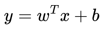
Where:
y represents the square footage value to be imputed.
x is a vector of observed features (like number_of_bedrooms, zipcode).
w is the weight vector learned from the regression.
b is the intercept term.
In practice, you might use a more powerful model (like a tree-based regressor) to capture nonlinear relationships. Once you have an imputed value for each missing entry, you incorporate those listings back into the primary dataset for training the main house price prediction model.
Strategy D: K-Nearest Neighbors Imputation
K-Nearest Neighbors (KNN) imputation locates the K most similar rows (based on features like neighborhood or property features that are not missing) and then uses their square footage values (e.g., an average of the neighbors’ square footage) to replace the missing entry. This method can preserve local structure in the data, but it can be computationally expensive for large datasets.
Strategy E: Multiple Imputation by Chained Equations (MICE)
Instead of filling missing values with single estimates, MICE repeatedly samples and imputes the missing values, generating multiple “complete” datasets. The final predictions are typically an aggregate (e.g., mean) of the results from each complete dataset. This approach captures uncertainty more effectively than simple one-shot imputation.
Practical Implementation Example
A brief Python pseudocode snippet illustrating model-based imputation:
import pandas as pd
from sklearn.ensemble import RandomForestRegressor

# Suppose 'df' is our pandas DataFrame with a column 'square_feet' that has missing values

# 1. Separate rows with known and unknown square footage
df_known = df[df['square_feet'].notnull()]
df_missing = df[df['square_feet'].isnull()]

# 2. Select features to predict square footage
features = ['bedrooms', 'bathrooms', 'lot_size', 'zipcode']  # example features
target = 'square_feet'

X_known = df_known[features]
y_known = df_known[target]

X_missing = df_missing[features]

# 3. Train a regression model (e.g., Random Forest) to predict square footage
reg_model = RandomForestRegressor(n_estimators=100, random_state=42)
reg_model.fit(X_known, y_known)

# 4. Impute missing values
missing_preds = reg_model.predict(X_missing)
df.loc[df['square_feet'].isnull(), 'square_feet'] = missing_preds
Evaluating Success of Imputation
Once imputation is done, it is crucial to assess how the imputation method influences downstream model performance. Overfitting or underestimation of variance could result if imputation is done naively. It is also advisable to retain an indicator feature to mark which rows had square footage imputed, allowing the main model to learn whether missingness is correlated with higher or lower housing prices.
Follow-Up Questions
How can we determine if the missing square footage values are truly random or systematically missing?
It is essential to conduct exploratory analysis. You can:
Investigate whether the missing entries correlate with particular neighborhoods, property ages, or price ranges.
Compare distributions of properties with and without square footage data. If houses missing square footage are noticeably older or from a less affluent district, the data are likely not missing at random.
Use statistical tests (like a chi-square test) to see if the missingness of square footage is linked to other categorical variables (neighborhood, for example). If significant relationships are found, the data are likely Missing at Random (MAR) or Missing Not at Random (MNAR).
When missingness is systematic, employing more advanced imputation (like a domain-aware imputation model) is better than simple mean-filling, as systematic absence can bias your price predictions.
Should we use a single imputation method or multiple imputation for this scenario?
This depends on factors like:
Size of the dataset: Large datasets often make multiple imputation feasible and more robust.
Complexity of missingness patterns: If missingness is correlated with other variables in intricate ways, multiple imputation by chained equations (MICE) typically offers a richer depiction of uncertainty.
Computational resources: Multiple imputation can be more computationally intensive, especially with 100K+ listings, but it may provide a more accurate representation of potential square footage values and thus yield better performance in the final house price model.
How do we validate that the chosen imputation method benefits the final price prediction model?
The end goal is to improve the predictive accuracy of the house pricing model. Hence:
Split your dataset into training and validation sets or use cross-validation.
Apply your chosen imputation technique only on the training fold, then measure how well the final model predicts prices on the validation fold. This step ensures that your imputation does not peek at the true test data.
Compare various imputation strategies (simple mean, median, regression-based, or multiple imputation) using the final evaluation metric (e.g., RMSE on house prices). The method that yields the best validation (or cross-validation) performance, while maintaining realism in the imputed values, is typically the optimal choice.
Is it possible that we could benefit from turning the presence/absence of square footage data itself into a feature?
Yes, indicating missingness as a feature can help capture subtle patterns. For instance, houses that omit square footage in listings might differ systematically (e.g., certain older properties may not list their square footage or certain neighborhoods might be less strict about listing details). By adding a binary feature such as “missing_square_feet = 1 if missing, else 0,” the model can learn to adjust predictions if missingness correlates with a higher or lower price bracket.
This approach is often especially helpful if the missingness is not purely random. In practice, combining an indicator feature with an appropriate imputation method can boost the accuracy of the final housing price model.
Below are additional follow-up questions
What are some scenarios where it might actually be acceptable to exclude the missing data rather than imputing?
One specific context could be if the total dataset is extremely large—say millions of rows—and dropping 20% still leaves a substantial amount of data. Even then, you would typically want to analyze the distributions and patterns of missingness to ensure that you are not discarding data in a way that systematically biases the model. For example, it may turn out that the 20% missing square footage entries are largely concentrated in certain neighborhoods or within older properties. If that is the case, excluding them might bias the model toward the types of homes that did have square footage recorded.
Another scenario is if your data science team suspects that the observations missing square footage come from an entirely different population (e.g., specialized housing types) that you do not wish to include in your modeling. In this edge case, you might intentionally drop them if the model’s usage context is specific to the non-missing data. Still, the key step is to verify that these missing points do not carry patterns important to your downstream prediction tasks.
A potential pitfall is that even in very large datasets, discarding 20% of records can lose rare but informative patterns—for instance, unusual yet valuable corner cases. If those corner cases end up being systematically absent, the model can fail for those same corner cases in real-world deployments, especially if prospective user data sometimes omits square footage for similar reasons.
What if square footage is only one of several features missing data? Does that change the imputation strategy?
When multiple features have nontrivial levels of missingness, a single imputation approach may not suffice. For instance, if both square footage and lot size are missing in 20% of the listings, you might need a more robust multivariate imputation technique such as Multiple Imputation by Chained Equations (MICE). This technique iterates over each feature with missing data in turn, regressing that feature on all the others, and imputes its missing values.
This iterative approach attempts to preserve the relationships among multiple features. A naive single-feature imputation (e.g., modeling square footage alone) can break correlations that exist between square footage and lot size, bedrooms, or other variables that may also contain gaps.
The risk here is that if you try to handle each missing feature in isolation, you might inject inconsistencies or unrealistic combinations (for instance, a large house on a minuscule lot, which might not be common in the real world). This can reduce the fidelity of your synthetic completions and degrade your final model’s generalization.
How can we avoid leakage of target information when performing imputation?
Data leakage arises if you use information from the target variable (in this case, the sale price or some transformation of it) to guide the imputation of square footage. In standard practice, you should not incorporate the final price (the label you are trying to predict) into the model used to impute missing square footage. Otherwise, your model can overfit by indirectly accessing that target signal during training.
One best practice is to partition the data into training and validation sets first. Then, fit the imputation model using only the training subset (without reference to the property price). After that, apply the fitted imputation pipeline to the validation set and eventually to the test set. This ensures that no target data from the validation or test sets bleed into the imputation process.
A subtle but important pitfall is that if you scale or normalize your features, you must compute the statistics (like mean or standard deviation) on the training set only, not the entire dataset. This same concept extends to any advanced imputation. The model for imputation should be derived from the training portion alone so that no knowledge of the validation or test sets leaks back into your pipeline.
What if the distribution of square footage changes over the three-year period?
Real-estate trends are not static. Construction practices can shift, new building codes might alter typical house sizes, and economic changes can favor either larger or smaller homes. If the distribution of square footage evolves over time, a single global imputation model might fail to capture time-specific trends. For instance, newer constructions in the last year of data might tend to have a larger average square footage, so imputing based on older data might systematically underestimate square footage in later listings.
One approach is to incorporate time or year of sale as a feature in your imputation model. Another is to create separate imputation models or separate reference statistics (for mean/median imputation) for each year or each quarter. This ensures the imputation respects the temporal distribution shifts.
A pitfall is that ignoring temporal variations can systematically bias your model, particularly if the test data reflect a distribution of house sizes that differ from historical listings. In that case, you might end up with biased predictions for the latest listings, which can undermine the entire model’s reliability in real-world deployments.
Does imputation risk artificially reducing the variability in the square footage feature?
Yes, any imputation approach can compress the true range of the data. For example, filling missing values with a mean or median tends to produce a cluster of “average-like” entries, which reduces variance and can alter the correlation structure between square footage and other features. Even advanced methods (e.g., regression-based or KNN) can introduce some shrinkage toward the typical range of square footage seen in the training data.
This can obscure genuine outliers—homes that are extremely large or small. If a property is genuinely unusual but had missing square footage, imputation might incorrectly produce a typical value, thus underestimating its uniqueness. A possible strategy is to maintain a record of imputed values and treat them with caution in subsequent analysis (e.g., weighting them slightly differently or ignoring them in certain steps if an outlier detection process is crucial).
A subtle consideration is whether the final predictive task might benefit or suffer from smoothing out outliers. Some models are sensitive to outliers and might benefit from reduced variance. Others, especially tree-based methods, may rely on the presence of these outliers to better split or partition the feature space for precise predictions.
How do we measure and reflect uncertainty in the imputed square footage values?
In many cases, it is valuable to estimate how certain or uncertain we are about an imputed value. For example, the range of plausible square footage for an upscale, older home in a historical district might be wide if the true distribution in that neighborhood is broad. Methods like multiple imputation (MICE) naturally reflect uncertainty by creating multiple plausible values. You then fit your final predictive model on each completed dataset and pool the results.
Another possibility is to use Bayesian regression models for imputation, which yield a posterior distribution over the missing feature. You can propagate this distribution into your main predictive model. This approach is more complex and can be computationally demanding with large datasets, but it offers a more nuanced understanding of the risk around each imputed value.
A pitfall is that you may fail to communicate imputation-driven uncertainty to downstream decision-makers. If the home price prediction model influences substantial financial decisions, not reporting the range of uncertainty for properties that had square footage estimated could mislead stakeholders. Transparent communication about confidence intervals or uncertainty bounds can help mitigate these risks.
What is the advantage of using domain knowledge during the imputation process?
Real-estate professionals often know that properties in certain neighborhoods have tight bounds on square footage, while others span a broad range. Additionally, domain knowledge about housing styles, zoning laws, or historical building codes can guide the plausible range for a property’s size. For instance, if there is a neighborhood built in the 1960s under a specific code, typical square footage might fall between 800 and 2,500. Knowing this, you can constrain the imputation model or design custom rules that reduce unrealistic guesses.
Sometimes, local ordinances or homeowner association rules might limit the minimum or maximum square footage. Implementing these constraints can increase imputation accuracy. Another real-world scenario is historical or cultural contexts, such as neighborhoods known for expansions or renovations. Such insights can be encoded as features or used to build specialized models for different segments of the data.
A pitfall is misapplying domain knowledge that does not accurately reflect the data at scale or using anecdotal evidence that contradicts the more general patterns in the dataset. Proper validation on a held-out set is crucial to ensure that any domain-driven constraints do not degrade predictive performance or introduce contradictory assumptions.
How might we handle extremely sparse data where multiple key features (not just square footage) are missing in a large fraction of rows?
In some datasets, you might find that certain listings are missing half or more of their features, including crucial ones like lot size, number of floors, and year of construction. In such extreme scenarios, standard single-feature imputation might not suffice. Multiple imputation techniques (like MICE) could still be used, but if the missingness is too high, you risk introducing significant noise and spurious correlations.
In these situations, a multi-pronged approach might be needed:
Clustering or segmenting properties based on available attributes, then imputing within each cluster to reduce heterogeneity.
Using feature engineering to create aggregate or proxy variables (e.g., combine neighborhood and number_of_bedrooms to estimate building type).
Considering specialized data-sparse modeling techniques, such as Bayesian hierarchical modeling where partial pooling can help fill in missing information across clusters.
A key challenge is that with extremely sparse data, your imputation model might not have enough information to reliably estimate the missing values. You also risk magnifying existing biases, because if your data are systematically sparser in certain subpopulations or neighborhoods, your imputation might systematically misrepresent those homes. Proper cross-validation strategies that simulate real-world missingness patterns become even more critical here.