ML Interview Q Series: How does Adam’s optimization method differ from basic Stochastic Gradient Descent?

📚 Browse the full ML Interview series here.

Comprehensive Explanation

Adam (Adaptive Moment Estimation) combines concepts from both Momentum and RMSProp to adaptively adjust the learning rate for each parameter, using first and second moments of gradients. Basic Stochastic Gradient Descent updates parameters in a more uniform way across all dimensions. Adam incorporates the idea of accumulating moving averages of the gradients and their squares, leading to different effective learning rates for different parameters.

One of the most essential aspects of Adam is that it maintains two moving averages: one for the gradients (often referred to as the first moment) and another for the squared gradients (the second moment). These averages are also bias-corrected to account for the initialization at the beginning of training. By contrast, basic SGD only uses the current gradient to perform the parameter update.

Adam’s Key Equations

Below are the core update rules for Adam. They highlight how exponential moving averages of the gradient and its square are maintained, corrected, and then used to update parameters. Let g_t be the gradient at time step t. Let beta1 and beta2 be the exponential decay rates for the first and second moments respectively. Let alpha represent the step size, epsilon a small constant for numerical stability, and theta_t the parameters at time step t.

Here m_t represents the first moment estimate. It is essentially a running average of the gradient. beta1 is typically close to 0.9. The term (1 - beta1) is the weight assigned to the current gradient g_t.

Since m_t is biased towards zero at the start (when t is small), this bias-correction is applied. This division corrects for the fact that m_t was initialized at zero.

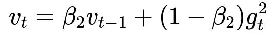
Here v_t is the second moment estimate. It is a running average of the squared gradient, capturing information about the variance of the gradients. beta2 is typically close to 0.999, making v_t smoother and more slowly varying.

This is the bias-corrected version of the second moment estimate v_t. Like m_t, v_t is also biased toward zero when t is small.

This final step shows how parameters are updated by subtracting a fraction of the bias-corrected first moment divided by the square root of the bias-corrected second moment, plus a tiny epsilon for numerical stability.

By contrast, a basic Stochastic Gradient Descent update looks like:

theta_{t+1} = theta_t - eta * g_t

where eta is the learning rate (often constant or decayed by a scheduled factor). In plain SGD, all dimensions share the same learning rate, and there is no direct mechanism to account for gradient variance in different dimensions unless additional modifications (like momentum or adaptive learning rates) are incorporated.

Why Adam Is Different and Potential Advantages

Adam applies different scaling factors to each parameter’s gradient, leading to adaptive per-parameter learning rates. Parameters with large gradients or with higher variance in gradients get appropriately scaled updates. This approach often leads to faster convergence in practice, especially for problems with sparse or noisy gradients.

Another key difference is that Adam’s bias correction steps help ensure that the moving averages do not remain artificially small during early iterations. This approach is especially helpful when training deep neural networks with large sets of parameters, because more stable updates often lead to smoother convergence.

SGD, on the other hand, remains a simpler technique and can sometimes generalize better under certain conditions—particularly if the dataset is large and well-scaled. With tuned hyperparameters (like momentum and well-chosen learning rates), SGD can still be extremely effective.

Potential Follow-Up Questions

Can you elaborate on the role of bias correction in Adam, and why it might be important?

Bias correction ensures that the exponential moving averages (m_t and v_t) are not underestimated during the first few iterations, when the initial values are zero. Early in training, because the algorithm is just beginning to accumulate gradient information, the raw estimates of m_t and v_t are systematically biased toward zero. The division by (1 - beta1^t) and (1 - beta2^t) corrects that bias so that the running estimates accurately represent the true first and second moments of the gradients even at the beginning of training.

If we omitted the bias correction, the updates might be too small and could slow down early training. The bias correction is especially critical when one wants consistent updates during initial epochs.

When might basic SGD perform better than Adam?

Although Adam often converges faster, plain SGD can sometimes achieve better generalization. In particular, when the loss landscape is smooth and the model has well-initialized parameters, SGD (with or without momentum) might avoid certain noise-induced pitfalls. Adam’s adaptive nature can occasionally overfit or converge to sharp local minima. Hence, some practitioners prefer to use Adam for rapid early training and then switch to SGD later, aiming for better generalization.

What happens if beta1 or beta2 are chosen poorly?

If beta1 is too large, then the first moment estimates might remain too persistent, causing sluggish updates in directions where the gradient has changed significantly. If beta2 is too large, the second moment estimates can overly smooth out the gradient variance, again slowing responsiveness to changes in gradient magnitude. On the other hand, if these values are too small, the moving averages fail to represent long-term trends, and the algorithm might behave erratically. Most implementations default to beta1 = 0.9 and beta2 = 0.999, which are generally robust choices.

What is the impact of epsilon in Adam’s update rule?

epsilon is a small constant added to the denominator to avoid division by zero. It also improves numerical stability when v_t or its bias-corrected counterpart is close to zero. This parameter typically takes a value like 1e-7 or 1e-8 in many frameworks. Large values of epsilon can result in more smoothing, while values that are too small can lead to numerical issues if the second moment is near zero.

Is Adam guaranteed to converge and how would you select an appropriate learning rate?

Adam is not guaranteed to converge for every possible scenario or objective function. Proper hyperparameter tuning (especially alpha, the main learning rate) is crucial. In many practical deep learning tasks, alpha is set in a range like 1e-3, with possible further tuning. While Adam often exhibits strong empirical performance, one must still experiment with different learning rates and sometimes schedule them to reduce over time. Lowering alpha during later epochs helps stabilize convergence and can improve final performance.

How would you implement Adam in PyTorch or TensorFlow?

Both frameworks have built-in Adam optimizers. For example, in PyTorch, you can implement Adam as follows:

import torch

model = MyNeuralNetwork()
optimizer = torch.optim.Adam(model.parameters(), lr=1e-3, betas=(0.9, 0.999), eps=1e-8)

for epoch in range(num_epochs):
    for x_batch, y_batch in train_loader:
        optimizer.zero_grad()
        predictions = model(x_batch)
        loss = loss_function(predictions, y_batch)
        loss.backward()
        optimizer.step()

All you need to do is specify the learning rate, betas for beta1 and beta2, and eps. This code snippet encapsulates all the logic of maintaining first and second moments of gradients, bias correction, and parameter updates.

Are there variants of Adam that address some of its shortcomings?

Several variants have been proposed, such as AdamW (which decouples weight decay from gradient-based updates) and AMSGrad (which modifies the second moment estimate to enforce a non-decreasing moving average of the squared gradients). These variants aim to improve convergence properties and generalization by tackling Adam’s tendency to overfit or fail in certain pathological cases. Their usage is situation-dependent, but they often provide stability in tasks where regular Adam might struggle.

Below are additional follow-up questions

Could the adaptive nature of Adam sometimes lead to overfitting, and how might we address this?

Adam adapts learning rates on a per-parameter basis by considering gradient magnitudes and their variances. While this can speed up training, one subtle pitfall is that the optimizer might adjust learning rates in a way that allows the model to fit noise in the training data more aggressively, leading to overfitting. This risk often increases if the learning rate alpha is too high or if the dataset is relatively small.

To address potential overfitting:

• Use regularization such as weight decay or dropout to constrain the capacity of the model.

• Deploy learning rate schedules that reduce alpha over time, preventing overly large parameter updates in later epochs.

• Employ techniques like early stopping, which monitors validation loss and stops training once the model starts to overfit.

A subtle real-world issue arises if the dataset is not only small but also noisy. In such cases, Adam’s adaptive steps can cause the model to latch onto spurious correlations. Mitigation includes standard data augmentation and cross-validation to ensure that the model does not converge to degenerate parameter configurations.

Is Adam always more memory-intensive than SGD, and why might this be problematic?

Adam requires additional memory for storing first and second moment estimates for every parameter, effectively doubling or tripling memory usage compared to basic SGD. This overhead is often acceptable for small or moderate networks but can be problematic in very large-scale models, especially those used in massive NLP tasks with hundreds of millions or even billions of parameters.

Memory constraints can lead to:

• Inability to train larger models on a single GPU or even a single multi-GPU system.

• Slower training due to increased data transfers between CPU and GPU when memory is oversubscribed.

• Potential out-of-memory errors that force training on smaller mini-batches, which can degrade the stability of gradient estimates.

A real-world scenario is large language model training, where memory optimization techniques (like gradient checkpointing) are sometimes used. In such cases, one might consider switching to more memory-efficient optimizers or specialized variants (e.g., Adam8bit) to handle massive parameter counts without requiring enormous GPU memory.

How does Adam behave under distributed or multi-GPU training, and what pitfalls might arise?

Under distributed or multi-GPU training, each device computes gradients on a subset of data (a shard of the mini-batch). These gradients are then aggregated (for instance, averaged) before parameter updates occur. Although Adam is straightforward to implement in distributed frameworks, certain pitfalls can occur:

1. Synchronization Overheads: Each GPU must synchronize its first and second moment estimates if all devices are to share the same values. This can be bandwidth- and latency-intensive.

2. Batch Size Variations: When scaling to many GPUs, the global effective batch size grows, which can alter Adam’s behavior. If the batch size becomes very large, the stochasticity of gradient estimates diminishes, possibly leading to different convergence properties than single-GPU setups.

3. Hyperparameter Sensitivity: Large-scale distributed training often requires retuning hyperparameters. Adam’s adaptive nature can become overly aggressive or too conservative when each GPU is dealing with a different part of the dataset.

In real-world scenarios, if the underlying distribution of data changes across workers (due to non-uniform data partitioning), the aggregated moment estimates might be skewed. Mitigations include proper data shuffling, repeated randomization of shards, and well-tested distributed training libraries that handle synchronization carefully.

When gradients are extremely sparse, does Adam still provide advantages compared to basic SGD?

Adam can still be beneficial for sparse gradient problems. Sparse gradients often arise in natural language processing tasks where embeddings for rarely occurring tokens receive updates infrequently. Adam’s per-parameter scaling (through second moment estimates) can help ensure that rare parameters receive meaningful updates when their gradients eventually appear.

Potential pitfalls:

• If the dataset is so sparse that many parameters almost never receive gradients, the moving averages for those parameters might be nearly zero for prolonged periods. This could lead to overly small or zero updates for rarely activated parameters.

• Tuning beta1 and beta2 becomes more critical, as extremely sparse gradients might require more aggressive momentum decay so that updates do not remain “frozen” for such parameters.

Real-world edge cases appear in large embedding tables, for example in recommender systems with millions of features. Carefully adjusting alpha and momentum-related hyperparameters is necessary to give rarely updated parameters enough chance to catch up.

What if the network has layers that vary widely in terms of gradient magnitudes—does Adam handle this better than SGD?

One of Adam’s strengths is its capacity to adapt the learning rate per parameter. In networks with certain layers (like embedding layers or attention layers) that produce very large or very small gradients, Adam automatically adjusts the update size. Parameters that have large gradients experience a proportionally reduced update, and those with small gradients experience a relatively increased update.

However, pitfalls can still arise:

• If the disparity in gradients is immense, even Adam’s adaptive adjustment might not fully normalize the updates, and some parameters could get stuck in regions of the parameter space.

• Layers that consistently receive smaller gradients might also be overshadowed, especially if beta2 is set too high and the second moment accumulates quickly.

In real-world architectures (e.g., GPT-like or BERT-like transformers), different layers may exhibit diverse gradient magnitudes. Adam helps to stabilize training across these layers, but thorough monitoring of layer-wise weight updates can reveal if certain layers are lagging behind.

How would you handle situations where Adam’s adaptive learning rate oscillates or becomes extremely small, making training stall?

Adam calculates effective learning rates through its ratio of first and second moment estimates. Oscillations can happen if the second moment (v_t) is slow to adapt to newly emerging gradient patterns, or if beta1 and beta2 values are poorly tuned relative to the problem. Training can also stall if the second moment grows too large, reducing the parameter update step size drastically.

To mitigate oscillation or stalling:

• Lower the beta1 or beta2 values slightly so that Adam is more responsive to recent gradient information.

• Use a decay schedule for the learning rate alpha to gradually reduce its value, smoothing out oscillations as training progresses.

• Reduce epsilon slightly if the denominator is too large, but be aware this can lead to numerical instability if it’s set too low.

A real-world edge case might involve cyclical or periodic data where gradients change direction or magnitude significantly across epochs (e.g., time-series problems with seasonal patterns). Tuning the momentum components or adopting a cyclical learning rate schedule can help reduce the likelihood of wild oscillations or extremely tiny updates.

Can we decouple weight decay from Adam’s gradient-based updates, and why would we do that?

A known shortcoming of many standard implementations of Adam is that weight decay is applied as part of the gradient term, effectively mixing weight decay with the adaptive moment computation. This can lead to inconsistent penalty application and, in some cases, poorer generalization.

AdamW is a popular variant that decouples weight decay from the adaptive gradient update step. In AdamW, weight decay is applied directly to the parameters before or after the gradient-based update rather than embedding it into the gradient itself. This separation ensures that weight decay is truly a regularization term, independent of the magnitude or direction of the adaptive gradient.

Potential pitfalls:

• Using standard Adam with a “weight decay” that’s actually implemented as L2 regularization might not behave the same as a pure weight decay approach, leading to confusion in hyperparameter tuning.

• If the weight decay factor is too large, one can still drastically degrade model performance, so it requires careful tuning even when decoupled.

Real-world scenarios: Large language models or vision transformers often rely heavily on AdamW to achieve better final validation accuracy and generalization performance. The decoupling helps maintain a more consistent penalization of large weights across layers.