
ML Interview Q Series: How does noise contrastive estimation define an alternative cost function and benefit large-scale modeling?


📚 Browse the full ML Interview series here.
Hint: NCE approximates the true likelihood by contrasting samples with noise.
Comprehensive Explanation
Noise contrastive estimation (NCE) is an approach to density estimation and model training that transforms the traditional maximum-likelihood estimation problem into a simpler probabilistic classification task. Instead of directly computing the normalization constant of a complex model (which is often expensive in high-dimensional or large-vocabulary contexts), NCE pairs actual data samples with artificially generated noise samples and trains a model to distinguish between them.
How NCE Defines an Alternative Cost Function
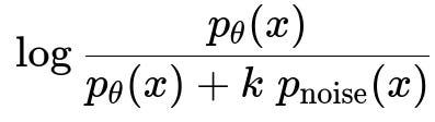
The idea behind NCE can be understood by viewing it as a binary classification problem. The model sees a sample x and attempts to classify whether x is drawn from the real data distribution p_data or from a chosen noise distribution p_noise. If we let p_theta(x) be the model’s unnormalized probability for x, and let k be the number of noise samples for each data sample, the probability that x is from the real data (rather than noise) can be written (in simplified text) as:
In this expression:
p_theta(x) is the unnormalized model probability of x. Typically, p_theta(x) = exp(score(x; theta)) in the log-linear or neural network context, where score(x; theta) is some learned function.
p_noise(x) is the noise distribution’s probability of x. Usually, this is chosen to be relatively simple, like a uniform or a known parametric distribution.
k is the ratio of noise samples to real samples; for instance, when we pair every real sample with five noise samples, k = 5.
When x actually comes from the real data distribution, the model is trained to maximize log( p_theta(x) / [p_theta(x) + k p_noise(x)] ). Conversely, if x is a noise sample, the model is trained to maximize log( k p_noise(x) / [p_theta(x) + k p_noise(x)] ). Summing these terms over all real and noise samples defines the alternative cost function. NCE effectively learns the normalization constant alongside model parameters, bypassing the need to compute the intractable partition function in typical maximum-likelihood estimation.
Why NCE is Beneficial for Large-Scale Embedding or Language Modeling Tasks
In large-scale language modeling or embedding tasks, calculating or sampling from the full distribution often becomes computationally expensive. Traditional softmax-based models (especially with very large vocabularies) require summations over all possible classes to normalize probabilities. This can be prohibitive when the vocabulary size is in the tens or hundreds of thousands.
NCE addresses this by reducing the normalization problem to a discriminative task. Instead of summing over all classes, the model only needs to contrast real samples with a manageable number of noise samples. This approach scales more efficiently because:
It avoids expensive normalization over a massive set of classes.
It can be implemented easily in neural frameworks (e.g., PyTorch or TensorFlow) by sampling from the noise distribution.
It converges more quickly in practice than naive maximum likelihood for large-scale tasks because it sidesteps heavy partition-function computations.
Practical Example of Using NCE for Word Embeddings
Below is a conceptual snippet showing how one might implement a simple noise-contrastive approach in Python-like pseudocode. Here, we assume we have a function get_noise_samples() that returns noise samples from p_noise, and a function get_real_samples() that returns real data samples from p_data. This is only a schematic example to illustrate the classification perspective in a training loop.
import torch
import torch.nn as nn
import torch.optim as optim

model = MyEmbeddingModel()  # Some embedding or language model
optimizer = optim.Adam(model.parameters(), lr=1e-3)
criterion = nn.BCEWithLogitsLoss()

for step in range(num_steps):
    real_samples = get_real_samples(batch_size)  # from p_data
    noise_samples = get_noise_samples(batch_size * k)  # from p_noise

    # Model scores for real samples
    real_scores = model(real_samples)  # unnormalized log p_theta(x)
    # Model scores for noise samples
    noise_scores = model(noise_samples)

    # Labels: 1 for real samples, 0 for noise samples
    all_scores = torch.cat([real_scores, noise_scores], dim=0)
    labels = torch.cat([torch.ones_like(real_scores),
                        torch.zeros_like(noise_scores)], dim=0)

    loss = criterion(all_scores, labels)
    optimizer.zero_grad()
    loss.backward()
    optimizer.step()
This kind of setup teaches the model to distinguish real samples from noise. With a sufficiently informative noise distribution and an appropriate choice of k, this effectively learns the underlying distribution without the burden of computing massive normalizing constants.
Common Follow-Up Questions
What is the Role of the Noise Distribution in NCE, and How Do We Choose it?
Choosing p_noise is crucial because the model’s ability to discriminate real samples from noise depends on how representative or tractable the noise distribution is. Common choices in language modeling include distributions proportional to the unigram frequency of words. Using a simple distribution (like a uniform distribution over vocabulary) can work, but might not always be optimal if the data distribution is highly skewed. A mismatch can slow convergence or lead to poorer estimates of the partition function.
How Does NCE Differ from Standard Maximum-Likelihood Estimation?
In standard maximum-likelihood estimation, the goal is to maximize p_theta(x) / Z(theta) for each sample x, where Z(theta) is the partition function. Calculating Z(theta) often involves summing or integrating over all possible samples, which can be intractable for very large domains. NCE avoids direct computation of Z(theta) by learning to classify between data and noise. This redefines the optimization problem without requiring explicit normalization over the entire sample space at each training step.
How Is This Related to Negative Sampling in Word2Vec?
Negative sampling in Word2Vec is essentially a specific instance of NCE. Word2Vec relies on a similar principle of discriminating real word-context pairs from noise word-context pairs. The difference is primarily in how the partition function is learned. In negative sampling, the partition function is often approximated or implicit, while in NCE there is an explicit parameter for the log of the partition function if one chooses to include it. In practice, both methods share the advantage of computational tractability in large-vocabulary scenarios.
Potential Pitfalls and Edge Cases
One pitfall involves the choice of k. If k is too small, the model may not adequately learn to discriminate data from noise, and if k is too large, training time might increase. Also, if p_noise is chosen poorly (for example, if it is too similar to p_data in a way that confuses the model), performance might degrade. In real-world tasks, a carefully tuned balance between the complexity of p_noise, the scale of k, and the available data is necessary to achieve stable, high-performing models.
Below are additional follow-up questions
Can NCE handle multi-class or multi-label settings beyond binary discrimination, and how do we adapt it?
NCE is generally formulated as a binary classification problem: real data versus noise. However, it can be adapted to multi-class scenarios by introducing a classifier that decides which class (including noise as one of the classes) a given sample belongs to. In this setup, instead of having a single binary output layer, one could use multiple outputs that represent each possible class plus an additional “noise” label. The underlying principle remains the same: the model still discriminates between real and noise samples, but now the real samples can come from multiple possible categories.
A potential pitfall arises if the multi-class transformation inflates the complexity of the task. The noise distribution needs to be well-defined for each class, so that the contrast remains meaningful. If the noise is trivially separable from only one class but not the others, the model may overfit or overemphasize discrimination between certain classes and noise rather than learning generalizable features. One must ensure that the ratio k and noise distribution are carefully chosen for each class to avoid data imbalance problems and maintain a fair comparison across different classes.
Does NCE guarantee convergence to the true data distribution, and under what conditions might it fail?
In principle, NCE can converge to the true data distribution under conditions such as having a flexible enough model family, a sufficient amount of training data, and an appropriate choice of noise distribution. The key theoretical requirement is that the noise distribution covers the support of the real data adequately. If the noise distribution has support that doesn’t overlap sufficiently with the real data distribution, the model might learn a distorted version of the partition function or misclassify boundary regions between real and noise distributions.
In practice, failure can occur if:
The model’s capacity is too limited. If the architecture cannot represent the underlying data distribution well, NCE’s classification objective may not capture all nuances.
The noise distribution is too different from the real data or does not capture enough diversity, causing the model to rely on overly simplistic discrimination cues.
The ratio k is too small or too large, leading to unstable gradients or insufficient contrast between noise and real samples.
Are there any typical convergence issues with NCE, and how can they be mitigated?
Convergence issues with NCE often revolve around imbalanced gradients, unstable updates, or poor coverage of the data by the noise distribution. When gradients are dominated by either real samples or noise samples (for example, if noise is trivially separable), training can stall or produce low-quality density estimates. Another challenge arises when the parameter that models the partition function update becomes unstable, causing oscillations in the estimated normalization constant.
Mitigation strategies include:
Keeping k at a moderate level so that neither real nor noise samples overwhelm the gradient updates.
Carefully choosing or tuning the noise distribution so that it overlaps sufficiently with the data distribution without being too trivial (e.g., pure uniform in a high-dimensional space).
Using stable optimizers (like Adam or RMSProp) with carefully tuned learning rates. Overly large learning rates can cause large oscillations in the normalization constant parameter.
Employing gradient clipping if the magnitudes of updates for the normalization parameter become too large.
Could NCE’s performance degrade if the model is overfitting or underfitting? How to handle these scenarios?
Yes. Overfitting with NCE might show up as the model perfectly discriminating real samples from noise samples without learning a robust estimate of the underlying data distribution. Underfitting might appear as the model being unable to discriminate well due to insufficient capacity or poor hyperparameter choices.
To handle these scenarios:
Regularize the model (via dropout, weight decay, or other methods) to avoid overfitting. Even though the main objective is a classification loss, the model can still memorize spurious patterns if it is excessively complex or if the noise distribution is too simple.
Increase model capacity or refine architecture if signs of underfitting appear (e.g., classification performance is poor on both training and validation sets).
Use validation sets of real and noise samples to measure how well the model generalizes. If real vs. noise discrimination on a validation set is not improving or saturates too early, it may signal overfitting or underfitting issues.
How do we evaluate the quality of the learned distribution or embeddings from NCE if we lack a ground-truth distribution?
Evaluation can be done indirectly using downstream tasks or proxy measures that reflect distribution quality. For language modeling, one might compute perplexity by approximating the partition function from samples or by evaluating how well the model predicts held-out text sequences in a next-token prediction scenario. For embeddings, one could measure performance on tasks like nearest neighbor classification, semantic similarity, or analogy tests (common in word embedding evaluations).
One subtle pitfall is that good discrimination (real vs. noise) accuracy does not always guarantee that the model captures every mode of the data distribution. A model might do well at classifying typical samples from the data and typical samples from the noise but still misrepresent rarer or more subtle regions of the data. Qualitative assessments or task-specific validations are often necessary to catch these blind spots.
What happens if the noise distribution is “too easy” to discriminate from the data distribution, and how do we address it?
If p_noise is very simple (e.g., a uniform distribution in a space where data is highly structured), the model may trivially distinguish data from noise. Training might then focus on superficial distinctions, failing to learn rich features that generalize to real-world tasks.
Addressing this typically involves making the noise distribution more challenging. One method is to choose p_noise that is somewhat similar to real data but still tractable. For instance, in language modeling, a noise distribution that mimics the unigram frequencies of words might be more challenging than a uniform distribution, forcing the model to learn more subtle discrimination. Another approach is to adopt a curriculum where p_noise gradually evolves from simple to more complex, ensuring the model’s decision boundary is continuously challenged.
How does self-normalized NCE differ from standard NCE, and what are the trade-offs?
Self-normalized NCE modifies the standard approach by introducing an additional constraint or objective that encourages the model’s unnormalized scores to sum (or integrate) to 1 over all possible outcomes. This removes the need to maintain an explicit parameter for the partition function, effectively baking normalization into the scoring function. A common approach is to penalize the discrepancy between the sum of exp(score(x)) over samples and the intended normalizing constant.
A major trade-off is computational overhead or complexity in the objective. While self-normalized NCE can simplify inference (because the scores are effectively normalized already), it can make training less stable if the penalty for normalization conflicts with the discrimination objective. Moreover, it requires careful tuning of the regularization strength that enforces normalization. If the penalty is too weak, the model may fail to be properly normalized, and if too strong, it can degrade performance by constraining the model’s capacity to discriminate real from noise.
Could we use a dynamic noise distribution that changes throughout training, and what are the benefits or pitfalls?
Adapting the noise distribution dynamically can help the model stay challenged as it improves. Early in training, a simpler noise distribution might suffice to guide the model. As the model gets better at discriminating, shifting to a more complex or realistic noise distribution can push the model to learn more detailed features.
Potential pitfalls include:
Tuning complexity: Deciding how quickly or frequently to update p_noise can be non-trivial. If the update schedule is misaligned, the training might become unstable.
Overlapping distributions: If the new noise distribution becomes too close to the real data too soon, the model might struggle to differentiate without adequate initialization, leading to poor or unstable gradient signals.
Implementation complexity: Generating dynamic noise samples might require additional data structures or sampling pipelines that complicate deployment.
What approaches can be used to efficiently parallelize or scale NCE for extremely large datasets or vocabularies?
NCE is often employed precisely because it scales better than traditional softmax approaches, but for extremely large datasets or vocabularies, further parallelization is necessary. Techniques include:
Distributed mini-batching: Split data across multiple workers, each generating noise samples and performing local gradient updates that are then synchronized.
Parameter server or collective communication frameworks: Store model parameters in a distributed fashion so that workers can access relevant parameters for local updates.
Caching noise samples or precomputing partial noise distributions to minimize the overhead of sampling in each step.
Using specialized hardware (GPUs, TPUs, or custom ASICs) that can handle large-scale matrix multiplications and large embedding lookups.
A subtle challenge is ensuring consistency when sampling noise across multiple workers. If different workers sample noise from different distributions or seeds, it could introduce bias or variance in the updates. Coordination or random seed management across workers is often necessary to keep training stable. Finally, memory constraints can become a bottleneck for storing embeddings or large model states, so partitioning or sharding embeddings is a common practice to keep memory usage manageable.