
ML Interview Q Series: How does the Adam optimizer, an extension of Stochastic Gradient Descent, operate in practice?

📚 Browse the full ML Interview series here.
Comprehensive Explanation
Adam (Adaptive Moment Estimation) combines ideas from momentum-based optimization and adaptive learning-rate methods such as RMSProp. It maintains an exponentially decaying average of past gradients (similar to momentum) along with an exponentially decaying average of past squared gradients (similar to RMSProp). This helps adapt the step size for each parameter, potentially accelerating convergence and smoothing out noisy gradient updates.
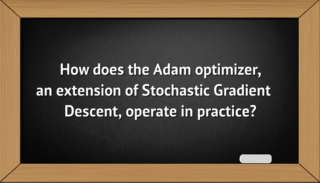
The method involves the following update steps:
Here:
m_t is the first moment estimate at iteration t.
beta_1 is a hyperparameter (commonly around 0.9) that controls the momentum decay rate.
m_{t-1} is the first moment from the previous iteration.
g_t is the gradient of the loss function at iteration t with respect to the parameters.

Here:
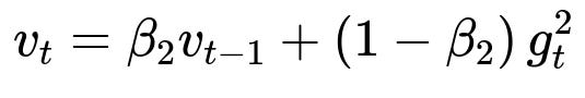
v_t is the second moment estimate at iteration t.
beta_2 is a hyperparameter (commonly around 0.999) that controls the decay rate for the moving average of squared gradients.
v_{t-1} is the second moment from the previous iteration.
g_t^2 is the element-wise square of the gradient at iteration t.
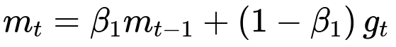
Because m_t and v_t are biased toward zero at the start of training (especially when t is small), Adam introduces bias-corrected estimates:
Here:
m_hat_t is the bias-corrected first moment estimate.
v_hat_t is the bias-corrected second moment estimate.
beta_1^t and beta_2^t are the exponential decay coefficients raised to the power t, which correct the bias introduced when the averages were initialized at zero.
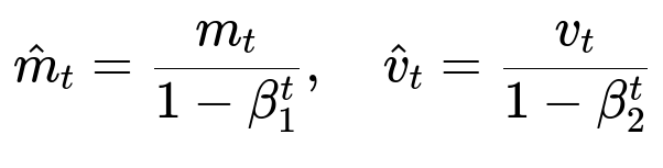
Finally, the parameters are updated as follows:
Here:
theta_t represents the parameters (weights) of the model at iteration t.
alpha is the learning rate.
epsilon is a small constant (e.g., 1e-8) added to the denominator to avoid division by zero and improve numerical stability.
Adam’s main advantage is combining the benefits of both momentum (to incorporate a notion of velocity) and per-parameter adaptive step sizes (to handle sparse gradients or different scales among parameters). This often leads to faster convergence in practice for a broad range of problems.
Key Properties and Practical Tips
Adam typically requires setting beta_1, beta_2, and epsilon. The default values (0.9 for beta_1, 0.999 for beta_2, and 1e-8 for epsilon) often work well. alpha should be tuned for specific tasks, although 1e-3 is a common starting point.
Users must watch out for overfitting and potential issues with non-convergent behavior if alpha or beta_1, beta_2 are poorly chosen. Despite the adaptivity, careful monitoring of model performance remains critical. In many deep learning frameworks, Adam is the default choice due to its robustness and ease of use.
Follow-Up Questions
Can Adam converge faster than standard SGD in all situations?
Adam often converges faster, especially early in training or for problems with sparse or noisy gradients. However, vanilla SGD might outperform Adam in some regimes, particularly for very large datasets and well-tuned learning rates, because plain SGD can sometimes find better minima in the long run. When momentum is added to standard SGD, performance can further approach Adam in many tasks.
How does one tune the beta_1 and beta_2 hyperparameters?
Typical values are around 0.9 for beta_1 and 0.999 for beta_2. They control the decay rates for first and second moments respectively. If gradients are very noisy, sometimes slightly higher beta_1 can stabilize updates, but setting beta_1 too high may slow adaptation to new gradient directions. For beta_2, values closer to 1.0 mean slower adaptation in the second moment but smoother estimates of the variance; occasionally, lowering beta_2 to 0.98 or 0.99 might help in specific tasks. The choice often depends on the scale and variability of gradients.
How does Adam compare to RMSProp or Adagrad?
RMSProp maintains a single exponentially decaying average of squared gradients and uses this for adaptive learning rates. Adam extends this by adding a momentum-like term for the first moment of gradients. Compared to Adagrad, which scales learning rates by the sum of squared gradients, Adam’s exponential averages ensure the scaling factor does not grow unboundedly over time, typically yielding more stable and consistent updates.
Why is epsilon important in the parameter update rule?
When the second moment estimate is extremely small, dividing by its square root can lead to very large parameter updates. Adding epsilon to the denominator ensures numerical stability and prevents extreme changes in parameters that could cause divergence or overflow. Even though epsilon is often very small (like 1e-8), it can have a large stabilizing effect.
Under what conditions might Adam fail to converge?
If the learning rate alpha is too large or if the combination of beta_1, beta_2 leads to unreliable moment estimates, the updates can become erratic. Another subtle point is that when dealing with very large batch sizes or highly non-stationary data, Adam’s estimates might lag behind abrupt changes in gradients. Proper tuning of hyperparameters and monitoring validation metrics are therefore critical to ensure stable convergence.
How do you implement Adam in Python?
Below is a simple outline of how one might implement Adam for a parameter vector theta and a function that computes gradients:
def adam_update(theta, grad, m, v, t, alpha=1e-3, beta1=0.9, beta2=0.999, eps=1e-8):
    m = beta1 * m + (1 - beta1) * grad
    v = beta2 * v + (1 - beta2) * (grad * grad)

    # Bias correction
    m_hat = m / (1 - beta1**t)
    v_hat = v / (1 - beta2**t)

    # Update parameters
    theta = theta - alpha * m_hat / (v_hat**0.5 + eps)

    return theta, m, v
One would initialize m and v to zeros and increment t each iteration. The shape of m and v must match theta. In practice, modern deep learning frameworks implement Adam internally, managing multiple parameter tensors automatically.
How can one measure Adam’s effectiveness?
Common ways to assess Adam’s effectiveness are monitoring the loss curve, validation performance, and training speed. One might compare final validation accuracy or training time to baseline optimizers like SGD or RMSProp. If performance is not satisfactory, hyperparameter tuning (learning rate, beta_1, beta_2) or switching to alternative optimizers might be considered.

Below are additional follow-up questions
How does Adam handle partial updates in a distributed training environment? Are there any pitfalls to be aware of?
In a distributed training setup, each worker typically computes gradients on a subset of the data (or a mini-batch) and then communicates these gradients (or parameter updates) to the other workers. Adam maintains internal state (the first and second moment estimates) that must remain consistent across all workers. Some common pitfalls include:
Non-synchronized State If each worker maintains its own m_t and v_t independently, discrepancies can arise if the workers do not effectively average or synchronize these moment estimates. One worker may end up taking larger steps than another if its estimated second moments differ significantly from the others. In asynchronous scenarios, this discrepancy can be amplified because updates might arrive out of order.
Increased Communication Overhead With Adam, each worker needs not just the raw gradients but also must keep consistent track of the running averages of gradients and squared gradients. If one tries to reduce communication overhead (e.g., by quantizing updates or doing local updates), it can harm the optimizer’s adaptive step logic.
Possible Instability with Stale Gradients If the system is asynchronous, some updates may be applied to a parameter that has already moved on in value. The staleness can degrade Adam’s bias corrections. Ensuring either synchronous steps or minimal staleness (e.g., using advanced distributed methods such as Hogwild or gradient accumulation with controlled synchronization) can help mitigate this.
An often-recommended approach is to synchronize the m_t and v_t values fully across all workers each iteration or after a fixed number of mini-batch updates. This ensures that each worker’s internal state remains consistent with the global state, preserving Adam’s theoretical underpinnings.
What is the difference between Adam and AdamW, and why might decoupled weight decay help for regularization?
AdamW is a variation of Adam that decouples weight decay from the gradient-based update. In standard Adam, adding weight decay is often done by adding a term lambda * theta (for some regularization coefficient lambda) directly to the gradient. However, this approach intertwines weight decay with Adam’s adaptive updates.
By contrast, AdamW applies weight decay as a separate step, effectively subtracting lambda * alpha * theta from the parameters, without feeding that term into the first or second moment estimates. This decoupling can lead to better generalization because the scaling of weight decay is not distorted by the adaptive gradients.
In practical terms:
Adam: Weight decay is added to gradients, so the adaptive moment estimates also incorporate weight decay contribution.
AdamW: Weight decay is done after the Adam update step, so the gradient is purely from the data, and the weight decay modifies the parameters directly.
By separating weight decay from the gradient calculation, AdamW ensures that regularization strength remains consistent regardless of the scale of the adaptive learning rate. This often gives more predictable and improved performance.
When is it beneficial to use half-precision training with Adam, and what issues could arise from underflow or overflow in the second moment estimates?
Half-precision (float16) training is beneficial for:
Large Neural Networks Modern deep networks with millions to billions of parameters can reduce memory usage significantly by using half precision. This often accelerates computation on GPUs that are optimized for mixed-precision or half-precision arithmetic.
Throughput Gains Half precision can increase computational throughput on specialized hardware (like NVIDIA Tensor Cores), allowing faster training without significant loss of numerical accuracy if managed properly.
Potential issues include:
Underflow in Gradients If gradients are extremely small, storing them in float16 may round them to zero, thus halting effective parameter updates for those dimensions.
Overflow in Accumulated Values The second moment v_t can become large if gradients are large, risking overflow in float16 representation.
Loss of Numerical Accuracy Even moderate imprecision can impact bias-correction steps. Typically, frameworks use mixed precision (keeping moment estimates in float32, while parameter updates and forward/backward passes might use float16) to mitigate such problems.
Maintaining the key accumulators (m_t and v_t) in a higher precision (e.g., float32) while using float16 for model weights is a common strategy. This helps keep Adam stable and prevents catastrophic underflow or overflow.
What is AMSGrad, and how does it address potential shortfalls in Adam’s second-moment estimates?
AMSGrad is a variant of Adam designed to handle scenarios where the adaptive learning rate (computed from the second moment estimate) can fluctuate abruptly and cause convergence issues. It introduces a "maximum" operation on the second moment estimates:
Instead of v_t being a raw exponential average that can decrease over time, AMSGrad maintains a maximum of the second moment estimates up to the current time step. This ensures that the denominator used in the update does not decrease, which can theoretically stabilize the parameter updates. When v_t is allowed to decrease, the effective learning rate can suddenly become too large, possibly leading to divergence or oscillations.
In practice, AMSGrad can provide more consistent convergence guarantees, though many applications still find vanilla Adam to work well enough. AMSGrad becomes more relevant when you observe training instabilities specifically linked to the second moment decreasing.
How can we incorporate gradient clipping in Adam, and what are the potential reasons for gradient clipping?
Gradient clipping is commonly used when training deep neural networks with Adam to avoid excessively large updates that can destabilize training. Here is the general approach:
Compute Raw Gradients The backward pass yields gradients g_t.
Clip Gradients One typical method is to clip the global norm: scale g_t so that its overall L2 norm does not exceed a predefined threshold (e.g., 1.0).
Adam Update Use these clipped gradients in Adam’s moment estimates, ensuring that large outliers do not blow up the second moment or cause extreme parameter changes.
Reasons for gradient clipping:
Exploding Gradients Certain architectures, like RNNs or very deep networks with poorly initialized parameters, can produce extremely large gradients. Clipping prevents updates that might cause parameters to become NaN or diverge.
Stable Learning By bounding gradient magnitude, gradient clipping forces more gradual changes and can serve as a safety mechanism while tuning learning rates, especially in the early stages of training.
Pitfalls include potentially oversuppressing gradients if the threshold is too low. This can slow down learning or mask legitimate large signals. Proper threshold selection often requires experimentation.
How do we effectively schedule the learning rate with Adam? Are there popular scheduling strategies that work well?
Although Adam adapts per-parameter learning rates, a global learning rate alpha remains a critical hyperparameter. Scheduling strategies can further improve performance:
Step Decay Lower alpha by a factor (e.g., 0.1) at specific epochs or intervals. This remains a simple and common approach.
Exponential Decay Multiply alpha by a factor like gamma^(epoch) or gamma^(iteration). This provides a smooth decay over time.
Warm Restarts or Cosine Annealing Gradually reduce alpha following a cosine function, then periodically "restart" to a higher value. This helps the optimizer escape local minima and sometimes yields better final convergence.
Cyclical Learning Rates Let alpha oscillate between lower and upper bounds. This approach can help Adam explore different regions of the parameter space.
In most deep learning frameworks, one might combine Adam with a scheduler object that updates alpha on each epoch or iteration. Monitoring validation metrics can guide when or how aggressively to lower alpha. Despite Adam’s adaptability, many practitioners see improvements by adding a schedule that reduces alpha as training progresses, helping refine convergence.
Under what conditions does Adam’s parameter update converge to stationary points that might not be minima, and how can we detect or escape these undesirable points?
Adam can, like many gradient-based optimizers, converge to "saddle points" or local minima that do not offer the best solution:
Plateaus in the Loss Surface In high-dimensional spaces, Adam might drift into regions where gradients are tiny but do not correspond to true global minima. This can happen if the second moment estimate becomes large, making the effective step size extremely small, or if the model’s gradient structure has many flat regions.
Vanishing Gradients In some architectures (e.g., very deep networks with certain activation functions), the gradients might vanish, and Adam’s moment estimates might keep the step size near zero on certain layers, causing a stationary but suboptimal point.
Detection:
Monitoring Validation and Training Curves If the training loss fails to decrease for many iterations but the validation loss remains high, the algorithm may be stuck in a poor stationary region.
Gradient Norm Checking if the gradient norm is consistently near zero while the training loss is still not minimal can hint at a poor local minimum or saddle.
Escaping Strategies:
Learning Rate Modifications Scheduling the learning rate or adding warm restarts can inject the necessary "jolt" to escape a plateau.
Random Restarts In some settings, re-initializing from different starting points might yield a better solution, although this is more common in smaller models.
Regularization or Architectural Tweaks Introducing skip connections or batch normalization can mitigate vanishing gradients, giving the optimizer a smoother, more navigable loss surface.