
ML Interview Q Series: How is the 68-95-99.7 principle relevant when describing a Normal Distribution?

📚 Browse the full ML Interview series here.
Comprehensive Explanation
The 68-95-99.7 principle, often called the "empirical rule," describes how data is distributed in a normal (Gaussian) distribution around its mean. For a normal distribution with mean mu and standard deviation sigma, it states that about 68% of the observations lie within 1 standard deviation from the mean, 95% lie within 2 standard deviations, and 99.7% lie within 3 standard deviations.
It relies on the properties of the normal distribution, which is symmetric about the mean and characterized by a bell-shaped curve. The precise shape and spread of the curve are determined by mu and sigma. Mathematically, the probability density function (PDF) for a normal distribution can be expressed as:

In this formula, mu is the distribution’s mean, sigma is the standard deviation, and x is any specific data point. The exponential term ensures that observations are most frequent around the mean, gradually decreasing in frequency (probability) as we move away from mu in both directions.
Centering our attention on the 68-95-99.7 rule:


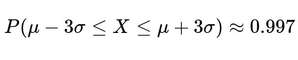
Here X is a random variable following the normal distribution. These intervals (mu ± k*sigma) show the range of values that X can take while maintaining a specific probability. Although the exact percentages are derived from integrating the PDF over those intervals, they are rounded to 68%, 95%, and 99.7% for simplicity and memorization.
The 68-95-99.7 rule is used extensively in statistical analyses and machine learning tasks, especially when judging how typical or extreme a data point is with respect to an assumed normal distribution of the data.
Example with Python Code
import numpy as np

np.random.seed(42)
mu = 0.0
sigma = 1.0
data = np.random.normal(mu, sigma, 10_000)

within_1_sigma = np.logical_and(data >= mu - sigma, data <= mu + sigma).sum()
within_2_sigma = np.logical_and(data >= mu - 2*sigma, data <= mu + 2*sigma).sum()
within_3_sigma = np.logical_and(data >= mu - 3*sigma, data <= mu + 3*sigma).sum()

print("Percentage within 1 sigma:", within_1_sigma / len(data) * 100)
print("Percentage within 2 sigma:", within_2_sigma / len(data) * 100)
print("Percentage within 3 sigma:", within_3_sigma / len(data) * 100)
Running this code typically yields results close to 68%, 95%, and 99.7% for 1, 2, and 3 standard deviations respectively.
Why It Matters in Practical Scenarios
This principle helps analysts identify outliers and assess variance within a dataset. For processes or datasets that are approximately normal, if a data point lies beyond 3 standard deviations from the mean, it might be an outlier or warrant special investigation.
It also allows for simpler rule-of-thumb calculations. For example, if you assume normality and want to predict coverage intervals around the mean without having to do complex integration of the PDF, you can rely on the 68-95-99.7 breakdown.
Potential Follow-up Questions
What if the data is not perfectly normal?
Real-world data can deviate from the perfect symmetry and kurtosis of a normal distribution. For instance, income distributions are often skewed. In these cases, the 68-95-99.7 rule may not hold exactly. Analysts might use alternative distributional assumptions such as log-normal, or they might employ non-parametric methods to evaluate intervals. Transformations like log transforms can sometimes bring the distribution closer to normal.
How can we tell if our dataset is normal enough to apply this rule?
Analysts can visually inspect histograms or Q-Q plots to see if the data resembles a bell curve. They can also perform statistical tests (e.g., Shapiro-Wilk, Kolmogorov-Smirnov) to check normality. If the dataset passes these checks, then the 68-95-99.7 rule might be a fair approximation. If not, more robust methods or distribution-free approaches could be employed.
Why are the numbers specifically 68, 95, and 99.7?
These specific percentages come from the properties of the cumulative distribution function (CDF) of the normal distribution. When integrating the normal PDF within 1, 2, or 3 standard deviations of the mean, it yields approximately 68%, 95%, and 99.7% coverage. The exact values to more decimal places are around 68.2699%, 95.4497%, and 99.7300%, but the rule rounds them for simplicity.
Could we use the 68-95-99.7 principle to detect anomalies?
Yes. In many anomaly detection systems that assume normality (for instance, Gaussian-based outlier detection), data points that fall outside 3 standard deviations may be flagged as anomalies. This is not foolproof for every application (some processes are multi-modal, highly skewed, or heavy-tailed), but for data that is well-approximated by a single Gaussian, the rule can be an effective heuristic.
Does the presence of outliers significantly affect the application of this rule?
Since the normal distribution is sensitive to extreme values, outliers can distort the estimated mean and standard deviation, thus making the 68-95-99.7 rule less reliable. A robust approach might include using measures less sensitive to outliers, such as the median and the interquartile range, or applying outlier filtering techniques first, then recalculating mu and sigma.
In what ways is this rule useful in Machine Learning?
Many machine learning algorithms rely on assumptions of normality in their components or in residuals (for instance, in linear regression, the residuals are often assumed to be normally distributed). The 68-95-99.7 rule provides a quick check on whether residuals or features follow the expected pattern. It also provides a guideline for normalizing data. If data is assumed normal, standardizing (subtracting the mean and dividing by the standard deviation) can help algorithms converge more reliably and identify unusual observations.
How does it help in evaluating model assumptions?
If you have a predictive model that presupposes normality in its error distribution, you can validate that assumption by plotting a distribution of the residuals. If they align reasonably with a normal shape, the 68-95-99.7 rule can be used to see if the residuals behave as expected. Deviations from these percentages might imply your model or distributional assumption is off.
Can this rule be generalized beyond three standard deviations?
While the classic rule highlights 1, 2, and 3 standard deviations, it can be extended further. For example, around 99.99% of normal distribution data is typically contained within about 4.4 standard deviations from the mean. However, most references stick to the simpler 1-sigma, 2-sigma, 3-sigma interpretation for day-to-day statistical reasoning.
How do we handle extremely large datasets?
For very large datasets that are normally distributed, the empirical estimates of mu and sigma tend to be more stable (due to the law of large numbers). Thus, the observed percentage of data within those standard deviations will tend to converge closer to 68%, 95%, and 99.7%. If the dataset is not normal, large sample sizes might still not fix the discrepancy, and in that case a different distribution or approach is necessary.
Below are additional follow-up questions
If the data distribution is severely multi-modal, does the 68-95-99.7 rule still make sense?
When data has more than one prominent peak (i.e., it is multi-modal), the assumption of a single, central mean with data points symmetrically spread around it no longer holds. A multi-modal distribution can be thought of as a mixture of multiple underlying distributions. In such scenarios, forcing the entire dataset into a single normal distribution can be misleading.
One pitfall is that the overall mean could lie somewhere between two (or more) modes where there’s very little actual data. The standard deviation calculated from this overall mean might not reflect how the data is truly clustered. Consequently, percentages like 68%, 95%, and 99.7% around this single mean are no longer valid indicators of typical spread.
A more robust approach is to identify each mode and treat each cluster separately. You might fit a mixture of Gaussians (e.g., via Gaussian Mixture Models) or employ a non-parametric density estimation approach. By doing so, each mode can be characterized by its own mean and standard deviation, providing more accurate coverage probabilities for each cluster.
Edge cases and pitfalls:
Some real-world processes might appear single-peaked but have a hidden secondary mode. If this is missed, applying the 68-95-99.7 rule can produce erroneous coverage estimates.
If the data is partially segmented (e.g., data from two different but overlapping populations), you can see a single peak with a “heavy shoulder,” which can still break normal assumptions without forming a distinct second peak. In such borderline scenarios, a unimodal assumption is risky.
How do we handle a situation where the data is truncated or censored?
Truncation and censoring mean that certain ranges of data are not observed or are only partially observed. For example, if measurements below a certain threshold are not recorded, the dataset is truncated on the lower end. Alternatively, if values above a certain threshold are all recorded as “just above threshold,” that’s censoring.
When data is truncated or censored, the observed distribution is not the true distribution. The assumption that the entire bell curve is represented is incorrect, so the standard empirical rule percentages might be off. For instance, if you have a lower bound truncation, the observed mean might shift upward, and the observed standard deviation may shrink compared to the true population.
In practice, methods such as survival analysis techniques (e.g., Kaplan-Meier estimates) or maximum likelihood estimation with truncated distributions can be employed. These approaches explicitly model the missing or censored portion of the data, allowing you to better infer the underlying distribution.
Edge cases and pitfalls:
Ignoring the truncation or censoring can lead to confidence intervals or coverage estimates that are drastically smaller or bigger than the true values.
If most of the data is within the truncated or censored range, you might falsely confirm that the data is following a neat bell curve, only to discover later that the tail beyond the threshold has been clipped.
Does the empirical rule apply if the data is discrete but we approximate it using a normal distribution?
Discrete data (e.g., counts of events) often come from distributions like Poisson or Binomial. For large enough counts and under certain conditions (e.g., mean is sufficiently large), the Central Limit Theorem can make a normal approximation reasonable. However, the fit is rarely exact, and small or moderate sample sizes can pose serious challenges.
If the discrete variable is well-approximated by a normal distribution, the 68-95-99.7 rule might be used as a rough guideline, but expect deviations in the tails. In particular, discrete distributions with strong skewness, or those that have a small mean, can produce skewed or heavily concentrated data that deviate from the symmetric bell shape.
Edge cases and pitfalls:
Very low event rates in a Poisson process: The distribution might be heavily skewed, so a normal approximation can badly misestimate the probability of events that are multiple standard deviations away from the mean.
Boundaries: Discrete data like the number of defective parts cannot go below zero, so the left tail is cut off, violating a key assumption of the unbounded normal distribution.
How does measurement error affect the validity of the 68-95-99.7 rule?
Measurement errors can inflate or distort the variance in your data, especially if these errors are not independent of the true measurement. If measurement error dominates the variation, the data’s distribution might appear wider, potentially making the standard deviation an overestimate of the true variability among underlying true values.
Additionally, if measurement error introduces a bias (shifting all measurements in a particular direction), your estimated mean is off, and coverage intervals around that mean may not correspond to the true coverage. In practice, you must account for measurement error when deciding whether you can treat your data as “true” observations from a normal distribution.
Edge cases and pitfalls:
Instrument limitations: If an instrument has a saturation point (e.g., it cannot measure values above a certain threshold), this artificially truncates or caps the data on one side.
Time-varying error: If the measurement process changes over time (e.g., calibration drift), the data distribution might systematically shift, breaking the assumption of a stationary normal distribution.
What happens if the distribution has heavier or lighter tails (leptokurtic or platykurtic) than the normal distribution?
Kurtosis measures how concentrated data is near the mean versus the tails. A leptokurtic distribution (high kurtosis) has heavier tails than a normal distribution, so extreme values are more frequent. In that scenario, the 68-95-99.7 coverage intervals might underestimate how many observations lie far from the mean, and you’ll see more outliers beyond 3 standard deviations.
Conversely, a platykurtic distribution (low kurtosis) exhibits lighter tails compared to a normal distribution, so outliers are less common. The empirical rule might overestimate how many points should fall in the far tails. In practical applications, one needs to measure kurtosis (and skewness) to assess how well the normal approximation might hold.
Edge cases and pitfalls:
Financial returns are a classic example of leptokurtic data: “fat tails” can cause the normal-based risk models to drastically underestimate extreme market moves.
Some distributions, such as the uniform distribution, are platykurtic and do not have the characteristic bell-shaped peak.
If there’s a mismatch between sample standard deviation and population standard deviation, how does that impact the rule?
The 68-95-99.7 rule hinges on knowing sigma, the standard deviation. In practice, we often estimate sigma from a sample. If the sample is too small or not representative, the sample-based sigma might differ significantly from the true population sigma. This mismatch leads to coverage intervals that do not reflect the real spread of the data.
Biases can arise if:
The sample is skewed or not random, leading to an underestimate or overestimate of sigma.
The sample size is too small, meaning your estimate of sigma has high variance.
To mitigate issues:
Use robust sampling methods (random or stratified) to approximate the population parameters.
If the sample is small, consider using distribution-free intervals or methods such as bootstrapping to gauge uncertainty in sigma.
Edge cases and pitfalls:
In real-world online systems, the population distribution might keep changing. A standard deviation estimated from historical data can quickly become outdated.
If you rely heavily on the empirical rule in a system with misestimated sigma (for example, in control chart processes), you’ll either overreact to normal fluctuations or underreact to real anomalies.
How should the 68-95-99.7 rule be adjusted when dealing with time-series data that exhibit drifting means or variances?
Time-series data often violate the assumption of a stationary mean and variance. For instance, a stock price might show a slow upward drift over time, or a sensor measurement might exhibit periodic fluctuations.
To use an empirical rule-like approach on time-series data, you can apply:
Rolling or moving windows: Recalculate the mean and standard deviation within a short window so that the immediate past data determines the interval. This helps capture local behavior if the mean or variance changes over time.
Detrending or seasonal decomposition: Remove trends or seasonality so that the residuals can more closely follow a normal distribution around zero with relatively stable variance.
Edge cases and pitfalls:
If the drift is sudden (e.g., abrupt shift in a manufacturing process), you may need a mechanism to detect regime changes instead of relying on a simple rolling window that might take a while to “catch up.”
If the variance itself is time-dependent (e.g., in financial volatility modeling), a single global sigma is not appropriate, and you might use models like GARCH that incorporate time-varying volatility.
For small sample sizes, is the 68-95-99.7 rule still valid?
When you have very limited data (e.g., fewer than 30 data points), the law of large numbers and central limit theorem do not ensure that sample mean and sample standard deviation will match the true population parameters. The normal approximation can thus be quite poor, and the exact proportions suggested by 68-95-99.7 may not hold.
Small-sample approaches may rely on:
The t-distribution, which accounts for additional uncertainty in the estimate of the standard deviation for small n. However, the t-distribution approach usually applies to estimates of means rather than coverage intervals of raw data points.
Bayesian methods that incorporate prior knowledge about potential distributions of data or standard deviations.
Edge cases and pitfalls:
If your small dataset has outliers, the sample standard deviation can become inflated, leading to overly wide intervals.
Overfitting can occur if you try to fit a normal distribution too precisely to a tiny sample.
Does the 68-95-99.7 rule help in high-dimensional datasets?
In high-dimensional spaces, data often exhibits phenomena like the “curse of dimensionality.” Distances between points can become less meaningful, and distributions of features can be complex. Even if each feature is individually normal, correlations among features might cause the joint distribution to deviate significantly from a simple multivariate normal.
While a multivariate normal distribution extends the univariate normal concept to multiple dimensions, the 68-95-99.7 principle is specifically a univariate coverage rule. The direct extension in higher dimensions (e.g., using Mahalanobis distance) can still be applied if the data is genuinely multivariate normal, but real-world high-dimensional data rarely satisfies this strictly.
Edge cases and pitfalls:
If only a subset of features follows a near-normal pattern while others do not, analyzing them all together using a single multivariate model can be misleading.
In practice, you might need dimension reduction (PCA, autoencoders) to identify the principal components that are approximately normal.
Can we use the rule to compare two different normal distributions with distinct means and standard deviations?
If you have two separate groups, each assumed to be normally distributed but with different means (mu1, mu2) and different standard deviations (sigma1, sigma2), the coverage intervals for each group will differ. One group might be more spread out or have a higher central value than the other.
You can apply the rule separately for each distribution:
For distribution 1, about 68% of the data should lie within mu1 ± sigma1, etc.
For distribution 2, about 68% of the data should lie within mu2 ± sigma2, etc.
However, directly comparing coverage intervals across different distributions can be tricky. Just because a value is within 1 standard deviation of one distribution’s mean does not mean it’s “comparable” to the other distribution, which might have a very different scale or center. An alternative is standardizing each distribution (z-scoring each group) so you can compare relative positions within each group’s own distribution.
Edge cases and pitfalls:
If the sample sizes for the two distributions differ greatly, your estimates of their parameters might differ in reliability.
If you suspect the two groups are drawn from the same underlying population, but your data says the means differ significantly, you need further statistical tests (like a t-test) rather than relying solely on the empirical rule for coverage overlap.