
ML Interview Q Series: How would you apply logistic regression, under the umbrella of supervised learning, to perform classification tasks?


📚 Browse the full ML Interview series here.
Comprehensive Explanation
Logistic Regression is a supervised learning algorithm frequently used for binary classification. While "regression" is part of its name, the output is not a continuous value but rather a probability of belonging to a certain class (often labeled as class "1" vs. class "0"). The algorithm models the log-odds of the probability that the target is in class "1" as a linear function of the input features.
The foundational idea behind Logistic Regression is to take a linear combination of input features and transform it with the sigmoid (logistic) function. If x is the input feature vector and w, b represent the parameters (weights and bias), then the probability of y=1 given x is:

Here:
p(y=1 | x) denotes the predicted probability of class 1 given input x.
w is the weight vector.
x is the input feature vector.
b is the bias term.
exp(...) is the exponential function.
Once we have this probability, we typically classify x as belonging to class 1 if p(y=1 | x) >= 0.5, otherwise we classify it as class 0.
Training Objective (Cost Function)
We train Logistic Regression by finding the parameters w and b that minimize the negative log-likelihood, often called the Binary Cross-Entropy Loss. For m training examples, the objective function J(theta) can be written as:
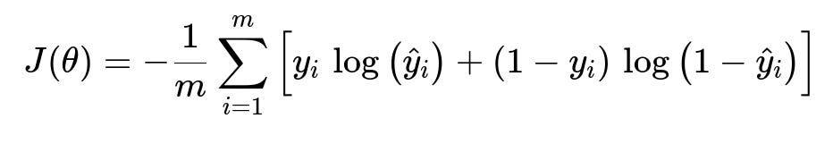
In this formula:
m is the number of training samples.
y_i is the true label of the i-th training example (0 or 1).
hat{y}_i is the predicted probability that the i-th training example is class 1.
theta is the set of parameters (w and b).
We typically use an optimization algorithm such as Gradient Descent (or variants like Stochastic Gradient Descent, Mini-batch Gradient Descent, etc.) to find the optimal parameters w and b that minimize this cost function.
Model Training Steps
Initialization: Initialize weights and bias, often with small random values or zeros.
Forward Pass: Compute the linear combination w^T x + b for each training example, then apply the sigmoid function to get the probability hat{y}_i.
Compute Loss: Use the binary cross-entropy loss function over all examples.
Backpropagation: Calculate the gradient of the cost with respect to w and b.
Parameter Update: Adjust w and b in the direction that lowers the cost.
Repeat until convergence or until a certain stopping criterion is met.
Decision Boundary
The logistic function outputs continuous values between 0 and 1, representing probabilities. A typical threshold of 0.5 is used to convert probabilities into class predictions:
If hat{y}_i >= 0.5, predict class 1.
Otherwise, predict class 0.
The decision boundary in the feature space is the set of points for which hat{y} = 0.5. Geometrically, this boundary is a hyperplane defined by w^T x + b = 0.
Advantages and Applications
Interpretability: Coefficients can be interpreted as how much each feature contributes to the log-odds of the prediction.
Efficiency: Training is typically fast and straightforward for lower-dimensional data.
Probabilistic Output: Provides class probabilities that can be useful for various tasks like ranking or threshold adjustment.
Example in Python
import numpy as np
from sklearn.linear_model import LogisticRegression
from sklearn.model_selection import train_test_split
from sklearn.metrics import accuracy_score

# Example dataset (X: features, y: labels)
X = np.array([[0.1, 0.3],
              [1.2, 3.1],
              [4.5, 2.3],
              [6.7, 8.2],
              [0.2, 0.1],
              [5.9, 2.1]])
y = np.array([0, 0, 1, 1, 0, 1])

# Split into train and test sets
X_train, X_test, y_train, y_test = train_test_split(X, y,
                                                    test_size=0.33,
                                                    random_state=42)

# Create and train the Logistic Regression model
log_reg = LogisticRegression()
log_reg.fit(X_train, y_train)

# Predict on the test set
y_pred = log_reg.predict(X_test)

# Evaluate
print("Predictions:", y_pred)
print("True labels:", y_test)
print("Accuracy:", accuracy_score(y_test, y_pred))
This snippet demonstrates training a Logistic Regression model on a small synthetic dataset. It outputs predicted labels, compares them with the ground truth, and calculates the accuracy.
What if the classes are imbalanced?
Real-world classification tasks often have class distribution skew. Logistic Regression can still be applied, but you must adjust decision thresholds, apply class weights, or oversample/undersample to handle imbalances effectively. Sklearn’s LogisticRegression provides a class_weight parameter to address such issues. Alternatively, using metrics like Precision, Recall, or F1-score instead of accuracy helps if the dataset has high class imbalance.
How do regularization and feature scaling affect Logistic Regression?
In practice, regularization (L2 or L1) is often employed to improve generalization by penalizing large weight coefficients. Feature scaling (e.g., standardization) often improves performance of gradient-based methods and can help the optimizer converge more quickly. L1 regularization can induce sparsity in the feature weights, effectively performing feature selection.
What happens if the data is not linearly separable?
Logistic Regression naturally models data with linear decision boundaries. If your data is not well separated by a linear boundary, performance might suffer. One can:
Engineer better features or transformations (e.g., polynomial features).
Use kernel methods (in some libraries that extend logistic regression to non-linear boundaries).
Move to more expressive models such as neural networks or other non-linear classifiers.
How do you interpret the coefficients?
Each coefficient in w indicates how much influence a corresponding feature x_i has on the log-odds of the outcome. A positive coefficient means increasing that feature value raises the odds of predicting class 1, while a negative coefficient lowers those odds. However, keep in mind that interaction effects are not explicitly modeled unless you add interaction features.
How do you handle overfitting?
Overfitting arises when the model fits noise in the training data. In Logistic Regression, overfitting can be mitigated by:
Using stronger regularization (larger regularization parameter if you are using the
Cparameter in sklearn).Reducing the number of features via feature selection or dimensionality reduction.
Acquiring more training data or applying data augmentation if applicable.
How do you extend logistic regression to multi-class classification?
By default, logistic regression covers binary classification. However, it can be extended to multi-class classification using strategies:
One-vs-Rest (OvR): Train a logistic regression model for each class vs. all other classes, pick the class with the highest probability in inference.
Multinomial softmax: Directly handle multiple classes by normalizing the linear activations for each class. Some libraries, such as sklearn, implement a “multinomial” option for logistic regression, internally applying a softmax function instead of a sigmoid.
What hyperparameters are commonly tuned?
In many standard libraries, some commonly tuned parameters include:
Regularization parameter (C in sklearn): Controls the strength of regularization (smaller C = stronger regularization).
Type of regularization (L1 vs. L2).
Solver (e.g., ‘lbfgs’, ‘sag’, ‘liblinear’): Each solver has different convergence properties and scales differently with data size.
How do you decide when to use Logistic Regression versus other models?
Logistic Regression is favored when:
You need clear interpretability of model coefficients.
You have a linearly separable or roughly linearly separable dataset.
You want a fast and robust baseline model.
You prefer a probabilistic interpretation and direct probability outputs.
It may not be the best choice when:
Your data exhibits complex, highly non-linear relationships.
You have an extremely large number of features and worry about overfitting (though regularization can help).
You can afford more complex models that might yield better predictive performance but at the cost of interpretability and training time.