
ML Interview Q Series: How would you compare and contrast the usage of Hidden Markov Models and Recurrent Neural Networks for tasks involving sequence data?


📚 Browse the full ML Interview series here.
Comprehensive Explanation
Hidden Markov Models and Recurrent Neural Networks both aim to deal with sequence data by capturing temporal dependencies. However, they differ significantly in their structure, assumptions, and capacities. Hidden Markov Models are built on explicit probabilistic foundations with latent states and Markovian assumptions. Recurrent Neural Networks, on the other hand, learn representations automatically from data using differentiable transformations over hidden states.
Hidden Markov Models
Hidden Markov Models use a hidden (latent) state space to model the dynamics of observable sequences. Each observed element in the sequence is assumed to be generated by an unobserved state, and state transitions follow Markov chain assumptions of first-order dependency. A key expression that captures the essence of a Hidden Markov Model is shown below.
Here, z_t is the hidden state at time t (in text form, z subscript t). x_t is the corresponding observation at time t. The model first draws the initial hidden state from p(z_1). Then, for each subsequent time index, the hidden state transitions from z_{t-1} to z_t according to a transition distribution p(z_t|z_{t-1}). Lastly, each observation x_t is generated from the hidden state z_t via p(x_t|z_t).
HMMs rely on dynamic programming algorithms such as the Forward-Backward procedure for efficiently computing probabilities of sequences and performing inference on latent states. Estimation of parameters (such as transition probabilities, emission probabilities, and initial state distributions) can be done via the Expectation-Maximization algorithm (the Baum-Welch procedure). Although HMMs can be extended to handle continuous observations (via Gaussian mixtures or other distributions) or more complex dependency structures (e.g., higher-order Markov chains or Factorial HMMs), these extensions can quickly become computationally cumbersome and may require strong assumptions about the data distribution.
Recurrent Neural Networks
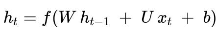
Recurrent Neural Networks (RNNs) learn to capture temporal dependencies through hidden state vectors that are updated at each timestep using neural network transformations. Instead of explicitly modeling transition and emission probabilities, RNNs discover a mapping from input data to hidden states in a data-driven manner. A fundamental recurrence relation for a simple RNN can be written:
Where:
h_t is the hidden state at time t.
x_t is the input at time t.
W, U, and b are learnable parameters (weights and biases) of the network (in text form, W, U, b).
f is an element-wise nonlinear activation function like tanh or ReLU.
By backpropagating through time (BPTT), RNNs learn parameter values that minimize a loss function appropriate for the sequence task, such as cross-entropy loss for classification or mean squared error for regression. RNN-based architectures do not assume any particular probabilistic structure a priori; they simply rely on gradient-based optimization to learn patterns from data. Variants like LSTM and GRU architectures incorporate gating mechanisms that help mitigate issues like exploding or vanishing gradients and allow for capturing long-range dependencies more effectively than standard RNNs.
Choosing Between HMMs and RNNs
Although both methods can handle sequential data, the choice depends on various factors:
Hidden Markov Models are favored when the underlying system can be well-approximated by latent discrete states with Markovian transitions and where interpretability of states and transitions is important. For small to moderate datasets, HMMs can be quite effective and easier to train. They also have a clear probabilistic interpretation.
Recurrent Neural Networks are typically chosen for complex sequence tasks (like language modeling, complex time-series forecasting, speech recognition) when large datasets are available, and you expect intricate or non-Markovian temporal dependencies. RNNs can capture more complex, high-dimensional relationships, but they often need more data and more computational resources, and they can be harder to interpret.
Simple RNN Code Snippet
Below is a minimal Python code snippet using PyTorch to illustrate how one might define a simple RNN layer for a sequence classification task. This example does not include the entire training loop but gives a sense of how an RNN is typically set up:
import torch
import torch.nn as nn

class SimpleRNNModel(nn.Module):
    def __init__(self, input_dim, hidden_dim, output_dim):
        super(SimpleRNNModel, self).__init__()
        self.hidden_dim = hidden_dim
        self.rnn = nn.RNN(input_dim, hidden_dim, batch_first=True)
        self.fc = nn.Linear(hidden_dim, output_dim)

    def forward(self, x):
        # x: shape (batch_size, sequence_length, input_dim)
        h0 = torch.zeros(1, x.size(0), self.hidden_dim)
        rnn_out, _ = self.rnn(x, h0)
        # Take the last hidden state
        out = self.fc(rnn_out[:, -1, :])
        return out

# Example usage
batch_size = 4
sequence_length = 10
input_dim = 8
hidden_dim = 16
output_dim = 2

model = SimpleRNNModel(input_dim, hidden_dim, output_dim)
sample_input = torch.randn(batch_size, sequence_length, input_dim)
logits = model(sample_input)
print(logits.shape)  # e.g., (4, 2)
How do HMMs and RNNs handle long-term dependencies?
Hidden Markov Models can be extended to higher-order Markov chains to capture somewhat longer-range dependencies, but the complexity and number of parameters grow, making them difficult to scale for very long sequences. Plain RNNs may suffer from vanishing or exploding gradients when dealing with long-term dependencies, but architecture variants like LSTM or GRU use gating mechanisms to better retain information across long intervals. In practice, these gating mechanisms allow RNNs to model much longer sequences than HMMs can handle without an exponential increase in complexity.
Potential Follow-up Questions
If the dataset is relatively small but there is still a need for a sequence model, which method might be more suitable and why?
A smaller dataset generally benefits from simpler models with fewer parameters, so an HMM might be a better choice if the assumptions about discrete latent states hold. HMMs require fewer parameters if the state and observation spaces are not large, and they have an interpretable probabilistic structure. By contrast, a complex RNN might overfit a small dataset without additional regularization or data augmentation.
Can we incorporate external knowledge into HMMs or RNNs?
It is straightforward to incorporate domain knowledge into HMMs by specifying transition probabilities or emission distributions that match known dynamics. For instance, if certain transitions are impossible, one can set those transition probabilities to zero. RNNs are more flexible, but it is harder to directly encode structured knowledge; they rely on learning from data. However, it is possible to inject constraints or external features as inputs or to regularize the network in certain ways. For real-world tasks that benefit from explicit knowledge (e.g., certain known state transitions in a biological process), HMMs can sometimes be more interpretable and simpler to constrain.
How would you extend an HMM or an RNN to handle continuous observation distributions for real-valued data?
HMMs can be extended by replacing discrete observation probabilities with continuous emission distributions, such as Gaussian or mixture of Gaussians. Parameter estimation still uses the EM algorithm, but now each emission probability is a continuous density. RNNs inherently accept real-valued inputs and produce real-valued hidden states and outputs by default, so they naturally handle continuous data. For tasks like regression, the output layer can be designed with a single neuron (or multiple neurons) and a linear or appropriate activation function. For tasks requiring generative capabilities with continuous outputs, variants such as RNN-based VAEs or normalizing flows can also be used.
What if the data has strong higher-order Markov dependencies?
Higher-order Markov dependencies in HMMs would require states that capture multiple historical observations (such as z_t depending on z_{t-1}, z_{t-2}, etc.). This leads to a combinatorial explosion of possible states unless carefully restricted. RNNs, particularly LSTMs and GRUs, can model these higher-order dependencies without exponentially increasing the number of parameters (although they still rely on enough data to learn them effectively).
Are there hybrid approaches combining HMMs and RNNs?
Yes, there are hybrid models that use the latent-state Markov chain foundation of HMMs but replace emission or transition distributions with neural networks. An example is a neural HMM where the emission probability is parameterized by a deep neural network. Another approach is using an RNN to predict transition probabilities in an HMM or to track the hidden-state posteriors in a learnable way. These hybrids retain the interpretability and probabilistic grounding of HMMs while benefiting from the representation power of neural networks. Such hybridization can be effective but also more complex to train and tune.
Below are additional follow-up questions
How do hidden states in HMMs differ from the learned hidden representations in RNNs, and how might this affect interpretability?
In a Hidden Markov Model, hidden states usually represent discrete latent factors that have a clear probabilistic meaning. Each latent state corresponds to a distinct regime or underlying condition, and the transition matrix indicates probabilities of moving between these states. This structure often facilitates interpretability because each hidden state can sometimes be tied to meaningful domain-related phenomena (for example, “rainy” vs. “sunny” states in a simplified weather model).
In Recurrent Neural Networks, the hidden states are continuous-valued vectors whose dimensions are not trivially interpretable. They are learned automatically via gradient-based training, and each component in the hidden state may encode nuanced aspects of the sequence history. Even though advanced interpretability methods exist (like attention visualizations in some sequence models), the hidden state is not typically associated with a single, explicit “label” or physical meaning. This can be a disadvantage if domain experts desire a clear explanation of each state. However, it also gives RNNs the flexibility to capture more complex relationships without adhering to a rigid set of discrete states.
A potential pitfall is assuming that an RNN’s hidden states function like an HMM’s discrete states. Analysts sometimes mistakenly try to force an interpretation on these continuous embeddings. They may attempt to cluster hidden states or treat each dimension as a stand-in for a specific phenomenon. Such attempts can be misleading if they disregard the model’s learned internal distribution or if the dataset is not large enough to learn reliable representations.
In situations where data might have missing observations in the sequence, how would HMMs and RNNs handle this challenge?
Hidden Markov Models can handle missing observations by integrating out the missing emission probabilities, thanks to their probabilistic formulation. The Forward-Backward algorithm can be adapted so that, for timesteps with missing values, the contribution of that emission is either skipped or replaced by a marginal probability. This approach works well if the data distribution assumptions (e.g., Gaussian emissions) are correct, or if we can reasonably define emission distributions for the missing data scenarios.
RNNs may struggle with missing data unless special preprocessing or architecture modifications are introduced. Common strategies include masking inputs to indicate which positions are observed vs. missing, or imputation strategies that fill in missing observations with estimates or placeholders. Some advanced RNN-based models incorporate gating mechanisms to handle irregularly sampled data or missing points (such as certain neural ODE or continuous-time RNN variants). However, these solutions tend to be more complex to implement and tune.
A subtle pitfall arises if missing data are not missing at random. For example, if sensor values fail under certain conditions that correlate with the target, naive imputation can introduce bias. With HMMs, an incorrect emission model for the missing data can yield systematically biased state inferences. With RNNs, if missingness is correlated with underlying states or outcomes, the network might learn spurious correlations unless carefully regularized or given explicit missingness indicators.
How does each approach scale in terms of memory usage and computational complexity as the sequence length grows?
For Hidden Markov Models, the forward-backward algorithm has a time complexity approximately proportional to (T * N^2), where T is sequence length and N is the number of hidden states. Memory usage typically scales with T * N when storing necessary intermediate quantities for the dynamic programming steps. If N is relatively small and T is large, HMMs can still be tractable, but the complexity may become substantial if N is large (e.g., hundreds or thousands of states).
For RNNs, the time complexity for a single pass through a length T sequence is roughly proportional to T * (cost of one timestep), where each timestep’s cost depends on the dimension of the hidden state and the network architecture (for instance, LSTM gating adds more parameters than a simple RNN). Memory usage can be high because backpropagation through time will store intermediate activations for each timestep. As T grows large, storing these activations may become problematic, though techniques like gradient checkpointing can help reduce memory requirements.
A subtle pitfall arises in extremely long sequences. For HMMs, if T is massive, even a small state space might pose large memory and computational demands when using naive dynamic programming. For RNNs, extremely long sequences can exacerbate vanishing or exploding gradients (unless gating or specialized architectures are used) and may also require large amounts of GPU memory for storing intermediate states during backpropagation.
How can we incorporate prior knowledge about state transitions or sequence structure in either model without overly constraining the learning process?
In Hidden Markov Models, prior knowledge can be introduced directly via the transition matrix and emission distributions. For instance, if it is known that certain transitions are impossible or highly unlikely, those transitions can be constrained. One can also place Bayesian priors on transition or emission parameters. This approach remains fairly interpretable and can reduce the effective parameter space when data is limited. However, excessive constraints can degrade performance if they are incorrect or overly rigid.
In RNNs, prior knowledge is less straightforward to encode, since the model is primarily learned via gradient descent. One approach is to embed known features or transformations as additional inputs at each timestep, effectively guiding the network toward using certain information. Another tactic might be to design specialized RNN cells that incorporate domain constraints (e.g., structuring gating functions to reflect known cyclical patterns). However, if the network is forced to adhere to incorrect constraints, the flexible data-driven approach is undermined.
A potential pitfall arises if domain knowledge conflicts with patterns in the data. HMMs with fixed transitions that do not align well with the real process may fail to fit the data and produce poor predictions. For RNNs, forcibly adding constraints that limit the hidden state dynamics could degrade the model’s capacity to learn. One must balance the desire for interpretability and domain-based structure with the model’s need to discover patterns.
What is the impact of state-space size on the representational power of HMMs compared to the hidden dimension of RNNs?
In HMMs, increasing the number of discrete states N increases the model’s representational power. More states allow for a finer partitioning of the observation space and more nuanced temporal dynamics. However, the parameter space and computational complexity also scale up. For instance, there are N(N-1) transition probabilities (minus constraints for normalization) and parameters for the emission probabilities. With too many states, overfitting can occur, and model estimation can become fragile unless large amounts of data are available.
In RNNs, increasing the hidden dimension can similarly increase the model’s capacity. Each additional hidden unit adds parameters in proportion to the dimensionality of the input and hidden vectors. This can capture more complex dependencies at the cost of higher risk of overfitting, more computational overhead, and possibly more challenging optimization. However, unlike HMMs, the representation is continuous and learned end to end, offering flexibility in how complexity is allocated among the hidden units.
A common pitfall is blindly increasing the state-space size in HMMs or the hidden dimension in RNNs, assuming it will automatically improve performance. Both approaches can overfit if not regularized or validated appropriately. Furthermore, a model with excessive capacity may become harder to interpret and tune.
In what scenarios might the Markov assumption in HMMs break down, and can we still use HMMs in those cases?
The Markov assumption stipulates that the probability of the next state depends only on the current state. Real-world sequences often violate this assumption, especially in language modeling or complex temporal processes where events can have dependencies spanning multiple timesteps. For example, in a speech recognition context, certain sounds may rely on context several phonemes back, which a simple first-order HMM might fail to capture.
Despite this, HMMs can still be used if the data partially satisfies the Markov property or if the violation is not severe enough to degrade performance. One common workaround is higher-order HMMs, where the next state depends on multiple preceding states. Another approach is to enlarge the state space to implicitly capture longer contexts, but this can explode the number of states. Alternatively, approximate factorization techniques (like Factorial HMMs) can help model more complex dependencies.
A pitfall arises if the data strongly violates the Markov property and the chosen HMM variant cannot approximate those long-range dependencies. One might attempt to add more states or adopt a higher-order model, but the parameter blow-up or computational overhead can make it impractical, leading to poor performance or infeasibility.
Could we deploy HMMs or RNNs in real-time systems where decisions must be made incrementally as data arrives?
Both HMMs and RNNs can be adapted to online or incremental scenarios. An HMM can be used in an online inference context by updating the forward probabilities at each incoming timestep and normalizing them. This yields a distribution over the hidden states in real time, which can then be used to make immediate predictions about the observation or the next state. Parameter learning in an online manner is possible but can be more complex (requiring incremental updates to transition or emission probabilities).
For RNNs, once trained, forward inference at each timestep is straightforward: we take the hidden state from the previous timestep, feed in the new input, and compute the updated hidden state to generate a prediction. Online training is more complicated because backpropagation through time typically requires unrolling over a fixed sequence length. However, certain truncated BPTT strategies can be applied in a streaming fashion.
A pitfall arises if the process generating data changes significantly over time (concept drift). An HMM or RNN trained offline may become out of date unless re-trained or updated online. For HMMs, one might adopt an online EM algorithm. For RNNs, one might perform repeated fine-tuning in small batches. Each approach adds additional complexity and must be carefully monitored for overfitting or catastrophic forgetting of older patterns.
How does each approach handle variable-length sequences, especially when comparing sequences of vastly different lengths?
Hidden Markov Models can naturally handle variable-length sequences through the same dynamic programming approaches (Forward-Backward). The computations scale proportionally with the length of each individual sequence. There is no fundamental requirement that all sequences be the same length. However, if some sequences are extremely short and others are extremely long, the model might struggle to share information across these very different cases, and the time or memory cost might be high for very long sequences.
Recurrent Neural Networks can process variable-length sequences by unrolling the network for as many timesteps as needed. In frameworks like PyTorch or TensorFlow, you can pack padded sequences to handle different lengths more efficiently. The main difference is that for RNN-based models, you often need to define a maximum sequence length if you are batching the data, but you can also handle unbatched data in a purely sequential loop for arbitrary lengths.
A pitfall occurs if the data distribution includes a few extremely long sequences that significantly affect training time or cause memory constraints for RNNs. With HMMs, very long sequences can still be processed, but the time cost of the Forward-Backward algorithm might be steep. For RNNs, large differences in sequence length within the same batch can lead to inefficiencies or gradient-related issues. Careful batching strategies or truncation/padding mechanisms can mitigate these concerns.
If you are dealing with multimodal sequences (e.g., audio + text + sensor readings over time), how can you integrate these different data sources into HMMs or RNNs?
In an HMM, integrating multiple data sources can be done by modeling the emission distribution as a joint distribution over all modalities. One might assume conditional independence given the hidden state (which is a common simplifying assumption), so that p(x_text, x_audio, x_sensor | z) factorizes into p(x_text | z) p(x_audio | z) p(x_sensor | z). Each modality’s distribution is then parameterized accordingly (e.g., discrete distributions for text tokens, Gaussian mixtures for continuous sensor data, specialized distributions for audio features). However, if the modalities are not conditionally independent given the state, further structure must be introduced, which can quickly become complex.
For RNNs, multimodal data can be concatenated or merged through specialized layers. For instance, you could embed text tokens, transform audio features via convolutional or recurrent layers, and then combine these processed features along with sensor readings into a single RNN. Alternatively, a separate RNN for each modality can feed into a joint layer. This approach leverages the representational power of neural networks to learn cross-modal relationships, but it may require extensive hyperparameter tuning.
A subtle pitfall arises if the modalities are at different sampling rates or exhibit different types of noise. HMMs can be extended to handle asynchronous modalities via separate Markov processes or hierarchical structures, but complexity grows quickly. RNN-based approaches can also struggle if one modality arrives more frequently than another, or if alignment is poor. Careful data preprocessing, synchronization, or alignment layers may be necessary to avoid learning spurious correlations or ignoring valuable signals.
Under what circumstances might a large RNN fail but an HMM succeed, and vice versa?
A large RNN might fail in scenarios where data is sparse, the Markov property is strongly valid, and interpretability of latent states is paramount. The neural network might overfit or fail to converge properly if the dataset is not large enough to learn the complex parameter space. In contrast, an HMM with carefully chosen discrete states and a small transition matrix might accurately capture transitions without overfitting.
Conversely, HMMs might fail when the real-world process violates simple Markovian assumptions, or when the data requires capturing complex, non-linear relationships that cannot be easily encoded in discrete state transitions. RNNs, especially LSTM or GRU variants, can excel at detecting patterns in high-dimensional data such as language models, where dependencies extend far beyond the immediate past.
A pitfall in practice is prematurely concluding that one approach is always superior. Some tasks might genuinely benefit from the interpretability and structure of HMMs (e.g., alignment tasks in computational biology where states correspond to known biological events), whereas others might require the raw predictive power of deep RNNs (e.g., complex language modeling with large vocabularies and long contexts). The “best” approach is heavily dependent on data complexity, domain constraints, available computational resources, and interpretability requirements.