
ML Interview Q Series: How would you choose the Loss Function for a Deep Learning model?


📚 Browse the full ML Interview series here.
Comprehensive Explanation
Choosing the right loss function is critical for training a deep learning model effectively. The loss function (also called the cost function or objective function) measures how well the model’s predictions match the true labels or targets. The optimization procedure iteratively adjusts the model’s parameters to minimize this loss, so the choice of loss function has a direct impact on how the model learns.
Different tasks call for different loss functions:
Classification tasks often use cross-entropy losses because these measure the divergence between the predicted probability distribution and the true distribution.
Regression tasks often use losses such as mean squared error (MSE), mean absolute error (MAE), or variations like the Huber loss.
Ranking or metric learning tasks may rely on contrastive or triplet losses.
Sequence-to-sequence tasks (e.g., language translation) can use cross-entropy with teacher forcing, or more specialized sequence-based losses.
Imbalanced classification might need focal loss or weighted cross-entropy to emphasize minority classes.
Specific considerations that influence your choice of loss function include the type of output layer, distribution of labels, robustness to outliers, interpretability, and computational constraints. In many real-world applications, the standard losses (cross-entropy for classification, MSE for regression) are a good starting point. However, specialized losses can be more suitable if the standard ones do not align well with your real evaluation metric or problem setup.
Common Loss Functions
For Classification
The most common choice for classification is cross-entropy loss, particularly softmax cross-entropy for multi-class classification and sigmoid cross-entropy (or binary cross-entropy) for binary classification. One typical binary cross-entropy loss function can be written as:

Where y_{i} is the ground truth label for the i-th sample (0 or 1 for binary classification), hat{y}_{i} is the predicted probability for the i-th sample, and N is the total number of samples in the batch. This formula penalizes the model heavily if it assigns a low probability to the true class. For multi-class problems, one usually sums over classes, using a softmax output layer.
When classes are highly imbalanced, you might add class weights to each term or use a focal loss variant. Focal loss focuses on hard-to-classify examples more than easy ones, making it effective for imbalance.
For Regression
A widely used loss function for continuous-valued predictions is the mean squared error (MSE). It is given by:
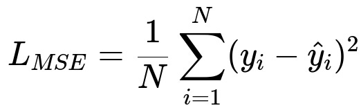
Where y_{i} is the true continuous target for the i-th sample, hat{y}_{i} is the model’s predicted value, and N is the total number of samples. MSE has a simple gradient that is easy to compute and interpret. But MSE can be sensitive to outliers, so in cases of heavy-tailed noise, mean absolute error (MAE) or Huber loss might be more robust.
Huber loss transitions from an L2 penalty to an L1 penalty beyond a certain threshold (delta). This limits the heavy penalty assigned to outliers, helping the model resist their influence.
Specialized Losses
Some deep learning tasks rely on specialized losses:
Hinge loss (often used in SVMs) for max-margin classification. Some deep networks also employ hinge-based objectives.
Contrastive loss and Triplet loss for learning representations in metric learning tasks. These drive pairs or triplets of embeddings to have desired distances in the latent space.
Reinforcement learning methods use reward-based objective functions rather than the typical supervised losses. Examples include policy gradients or actor-critic losses.
Sequence learning tasks can involve cross-entropy over time steps, attention-based alignment losses, or custom translation metrics (e.g., BLEU-based approximations).
Practical Implementation Example
Below is a simple example showing how one might implement a custom mean squared error (MSE) loss in PyTorch:
import torch
import torch.nn as nn

class CustomMSELoss(nn.Module):
    def __init__(self):
        super(CustomMSELoss, self).__init__()

    def forward(self, predictions, targets):
        # predictions and targets are tensors of shape [N, ...]
        return torch.mean((predictions - targets)**2)

# Usage in a training loop
model = SomeDeepModel()
criterion = CustomMSELoss()
optimizer = torch.optim.Adam(model.parameters(), lr=1e-3)

for data, labels in dataloader:
    optimizer.zero_grad()
    outputs = model(data)
    loss = criterion(outputs, labels)
    loss.backward()
    optimizer.step()
In this example, the predictions and targets are simply subtracted, squared, and averaged. This is functionally the same as PyTorch’s built-in nn.MSELoss. Custom losses can incorporate additional terms such as regularization or domain-specific constraints.
Balancing Theory and Practice
In practice, the model and the loss function are tightly coupled:
Output layer determines whether your model outputs probabilities, unbounded real values, etc. Ensure the loss function matches.
Evaluation metric for your real-world task might be something other than the chosen training loss. For instance, you might train with cross-entropy but measure F1 score. It’s common to see a mismatch between training loss and final performance metric; sometimes you might design or weight the loss function to approximate that final metric more closely.
Regularization may be integrated directly into the loss function (e.g., L2 or L1 penalty on parameters) or handled separately in certain frameworks. These techniques influence training stability and generalization.
Models learn what the loss function tells them to learn. If the chosen loss does not align well with business objectives or the final metric that matters (like precision, recall, or ranking), you may need to customize it.
Potential Follow-up Questions
What if my dataset is extremely imbalanced?
You can modify the cross-entropy loss by applying class weights or use specialized variants like focal loss. Class weighting gives more penalty to the minority class mistakes. Focal loss adds a modulating factor to the cross-entropy that emphasizes hard-to-classify examples. You might also see oversampling or undersampling techniques used in conjunction with these adjusted losses.
How do I handle noisy labels or outliers when choosing a loss?
Using more robust losses can help. For regression tasks, mean absolute error or Huber loss is less sensitive to outliers than mean squared error. For classification tasks, label smoothing can help mitigate overconfidence on noisy samples. You can also incorporate dropout or other forms of regularization. These strategies make the model less prone to overfitting erroneous labels.
Can I directly optimize my real-world metric (e.g., accuracy, F1 score)?
Some metrics, like accuracy, are not differentiable, so they are not directly usable as a gradient-based objective. Methods such as reinforcement learning or gradient estimators can sometimes circumvent this, but in most standard supervised settings, we resort to differentiable proxies (e.g., cross-entropy). However, you can monitor the non-differentiable metric on a validation set and potentially implement specialized gradient approximations or structured losses (for example, structured SVM approaches for certain ranking or structured prediction tasks).
Is there a unified approach to selecting a loss function?
There is no single universal approach, but here is the typical process: Understand your problem type (classification, regression, etc.), the nature of your target distribution (continuous, discrete, skewed, multi-label, etc.), the effect of outliers, and the evaluation metric you care about. Then select a known, well-tested loss function that aligns most closely with your scenario. Conduct experiments and, if needed, refine or customize.
How do I test if a custom loss function is working correctly?
A best practice is to start with a small synthetic dataset where you know the exact behavior you expect from the model. Ensure that your custom loss causes the model to behave in the anticipated direction. Debug step-by-step: check gradients, watch if the loss consistently decreases, and confirm that the outputs converge toward the known targets. Once it behaves as expected on the toy dataset, try it on more realistic data.
By methodically aligning the loss function with your problem requirements, distribution characteristics, and final performance metrics, you can make a well-informed choice and significantly improve your deep learning model’s effectiveness.
Below are additional follow-up questions
If my data distribution changes frequently, do I need to adjust the loss function?
When your underlying data distribution shifts (a phenomenon often referred to as dataset shift or domain shift), the model may struggle to generalize if its original assumptions are violated. A common pitfall is continuing to use a loss function tailored to the original distribution. Depending on how the distribution changes, you might need to modify how you weight examples or adjust certain hyperparameters in your loss.
For instance, if you were originally using cross-entropy for a balanced classification task, but the class distribution changes drastically (one class becomes very rare), you might suddenly find your model ignoring the minority class. Adapting by introducing class weights or switching to a loss like focal loss can help. In addition, when real-time streaming data is involved, you may need more dynamic strategies like online learning or periodically retraining and adjusting your loss function parameters to reflect new conditions.
A subtle challenge arises when only a subpopulation changes. For example, in a regression scenario where certain extreme values become more common, an MSE-based approach might amplify the influence of these outliers. In these cases, switching to a more robust alternative like mean absolute error (MAE) or Huber loss can mitigate the disruption from changing data patterns.
How can I incorporate domain knowledge directly into the loss function?
In many applications, domain knowledge can significantly improve model performance if encoded properly. One approach is to add custom penalty terms to the existing loss. For example, if you know that certain predictions must never exceed a certain threshold for safety reasons, you can add a penalty term each time the model’s output breaches that boundary. Another approach might be to structure the output layer so that it captures physically meaningful constraints—for example, predicting only non-negative values for quantities that cannot be negative.
An edge case to watch out for is over-constraining the model with domain knowledge. Too many rigid constraints can make training infeasible if the model is punished in every direction it tries to learn. It’s also possible that domain assumptions are incomplete or approximate, causing your extra penalty terms to lead the model astray. A common strategy is to use a “soft” penalty rather than a hard-coded threshold—this allows the model to occasionally violate constraints when it significantly benefits the overall performance.
What if I have a multi-label classification problem with overlapping labels?
In a multi-label problem, a single instance can belong to multiple classes simultaneously (e.g., an image that can contain both “cat” and “dog” labels). Standard softmax cross-entropy is not suitable here because it enforces the assumption that one instance belongs to exactly one class. Instead, you typically use a sigmoid cross-entropy formulation—applying a sigmoid activation for each label independently and summing up the binary cross-entropy terms.
A subtle issue in multi-label scenarios is the degree of label correlation. If labels frequently co-occur, standard independent binary cross-entropy might underexploit these relationships. You can address this with structured or graph-based losses that incorporate label-dependency information. One pitfall, however, is that such sophisticated losses can become more complex to implement and might require more data to learn label co-occurrences effectively.
How should I pick a loss for image segmentation tasks?
In image segmentation, each pixel (or voxel in 3D medical imaging) is assigned a class label. The popular choices are cross-entropy or dice coefficient–based losses. Cross-entropy is straightforward—apply it pixel-wise and average over all pixels. However, if the foreground object is small relative to the background, the dice loss (or a combination of dice loss and cross-entropy) can be more effective. Dice loss directly measures overlap between predicted and true masks, which helps combat class imbalance in segmentation tasks.
An important edge case is multi-class segmentation. You can generalize cross-entropy or dice loss to handle multiple classes, but you need to ensure that the total probability across all classes at each pixel is properly normalized if you are using softmax-based segmentation. Another issue is that if some classes are extremely rare, the model might learn to ignore them when only cross-entropy is used. In such scenarios, you might weight classes or use specialized focal/dice variants that emphasize underrepresented structures.
How can I incorporate fairness or interpretability constraints into my loss?
Fairness and interpretability are increasingly crucial in modern AI systems. One way to encourage fairness is to add a penalty term that measures disparities across protected groups. For instance, you might measure differences in false-positive rates among subgroups and penalize the model if those differences exceed a certain threshold. Another approach is to train a model to minimize a standard loss while constraining or penalizing group-level biases.
A real-world pitfall is the complexity of fairness definitions: many can conflict with one another. For example, optimizing for equal opportunity might hurt demographic parity. Consequently, you may have to balance multiple fairness criteria and standard accuracy or cross-entropy. This can complicate training since each fairness penalty might slow convergence or produce trade-offs that are not trivial to resolve.
Are there numerical stability concerns with certain loss functions?
Yes. Numerical stability can be an issue in large-scale deep learning. For instance, when computing log probabilities in cross-entropy, a predicted probability near zero can cause an overflow in the log function. Frameworks like TensorFlow or PyTorch typically provide numerically stable implementations of cross-entropy by combining the log operation with the softmax or sigmoid to avoid intermediate values that are too large or too small.
A similar concern arises in losses like hinge loss or exponential losses used in boosting, where large negative margins can cause exponential terms to blow up. Gradient explosion can also occur if you feed extremely large errors back through the network. To handle these scenarios, you often rely on built-in stable implementations or clamp values to prevent extremely large or small floating-point numbers. Careful initialization and gradient clipping can also mitigate stability issues.
How does the reconstruction loss in autoencoders or VAEs affect the learned representations?
For standard autoencoders, the reconstruction loss is typically MSE or MAE, comparing the input and the reconstruction. MSE encourages a more “smooth” reconstruction, while MAE might preserve edges or high-frequency details better. For variational autoencoders (VAEs), the loss is a combination of a reconstruction term (often MSE or cross-entropy if inputs are in [0, 1]) plus a Kullback-Leibler (KL) divergence term that regularizes the latent distribution to be close to a chosen prior distribution.
Because the KL term can dominate, you must tune the relative weight of the reconstruction and KL components. A common pitfall is placing too much emphasis on the KL divergence, causing the model to ignore the input data (posterior collapse). Conversely, if the KL term is too small, the learned latent space may fail to generalize and not act like a proper distribution. Balancing these terms is key to producing stable and meaningful generative performance.
Which loss function is best for time-series forecasting?
For many time-series forecasting tasks, MSE and MAE are the go-to starting points. MSE is commonly used, but it heavily penalizes large errors. MAE can be more robust if your time-series has outliers such as sudden spikes or unexpected events. In some industries, other custom metrics might apply. For instance, if the cost of underestimating demand is different from overestimating demand, you might incorporate an asymmetric penalty (like quantile loss) that places more emphasis on one side of the error distribution.
A major edge case is when your time-series patterns change over time (non-stationarity). A single error metric might no longer capture performance well across different regimes. Some practitioners dynamically adjust the loss to reflect more recent data or incorporate weighting that emphasizes recent observations. Another subtlety is that if your time-series can have zero or near-zero values, a log-based transformation in the loss can cause numerical challenges (e.g., taking log(0)). In those cases, you must carefully preprocess the data or choose a different approach for error measurement.
How do I verify my custom loss function during training so it doesn’t degrade performance unexpectedly?
When you introduce a custom loss, you risk bugs or misalignment with your actual objectives. A best practice is to start with a very small synthetic dataset where the correct outputs are trivially known. This allows you to confirm that the loss consistently decreases and that your model converges toward the correct solution. Checking intermediate gradients is also beneficial—look at the gradient values and confirm they have the expected sign and magnitude.
A more subtle issue is that even if your custom loss is mathematically correct, it might conflict with your final business or evaluation metric. For example, you could optimize a custom penalty that inadvertently reduces the model’s overall accuracy. Monitoring multiple metrics, not just the training loss, helps catch these misalignments. If you see your final performance metric worsening while your custom loss goes down, it may signal that your auxiliary penalty is too strong or the training objective needs to be rebalanced.