
ML Interview Q Series: How would you choose between using Random Forest and Gradient Boosted Trees for a specific problem?

📚 Browse the full ML Interview series here.
Comprehensive Explanation
Random Forest and Gradient Boosting Trees are two of the most widely used ensemble methods that rely on decision trees as their base learners. Both aim to aggregate multiple weak learners (decision trees) in different ways to produce a more powerful model.
Random Forest typically averages the predictions of many independently trained decision trees. Each tree is usually trained on a bootstrap sample of the dataset (bagging) and uses only a subset of features at each split. This approach helps reduce variance and mitigate overfitting.
Gradient Boosting Trees, on the other hand, train decision trees in an iterative fashion, where each new tree is fitted to the errors (or gradients of the loss function) of the previous ensemble. This additive and sequential nature often leads to higher predictive accuracy but can make the model more susceptible to overfitting if not carefully regularized.
Comparing Core Mathematical Formulations
Below is a key formula for Random Forest in a regression setting, where the final prediction is the average of predictions from B decision trees.
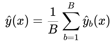
Here:
B is the total number of decision trees in the forest.
x is the input feature vector.
y_b(x) is the prediction from the b-th decision tree.
For Gradient Boosting, the model is built sequentially. One of the well-known formulations of an additive model is shown below, where each new tree is added to reduce the existing residuals.

Here:
F_m(x) is the boosted model after m iterations.
F_{m-1}(x) is the model trained up to iteration m-1.
h_m(x) is the new decision tree learned at iteration m.
gamma_m is a scaling factor derived from line-search or analytical solutions.
nu is the learning rate, which shrinks the contribution of each new tree.
Key Considerations for Choosing Between the Two
Performance and Accuracy In general, Gradient Boosting can outperform Random Forest in many tasks, especially if hyperparameters are well tuned. Its sequential nature allows it to focus on difficult training examples. However, Random Forest is still highly competitive and often easier to tune, so it might yield comparable performance in many practical scenarios.
Training Time and Complexity Because Gradient Boosting is built iteratively, it can take longer to train, especially for large datasets. Random Forest trains all trees in parallel (in principle), making it potentially faster to fit, though the number of trees in a random forest can also affect training time.
Sensitivity to Hyperparameters Gradient Boosting typically has more parameters to tune, such as the number of estimators, the learning rate, the tree depth, and regularization terms (subsample rates, column subsampling, etc.). Random Forest has fewer critical hyperparameters, typically just the number of trees, the maximum depth of each tree, the number of features to consider for each split, and minimal leaf size or similar stopping criteria.
Risk of Overfitting Gradient Boosting has a higher risk of overfitting if not regularized properly (learning rate, subsampling, and early stopping can help). Random Forest, by construction, is often more robust to overfitting thanks to bagging and feature randomization.
Interpretability and Diagnostics Both methods are ensembles of trees, so they are not as transparent as a single decision tree. Tools such as feature importances or SHAP values can help interpret both. Gradient Boosting’s sequential nature can sometimes make it trickier to interpret how each tree contributes to the final model.
Practical Considerations
Data Size Random Forest can handle large datasets more easily without extensive hyperparameter tuning. Gradient Boosting can still work well on large datasets, but tuning might be more expensive.
Imbalanced Data or Specific Loss Functions Gradient Boosting can be adapted to custom loss functions (like ranking losses or specialized versions of logistic loss for imbalanced data). Random Forest is generally used for standard regression or classification tasks, though it can handle class weighting.
When You Have Little Time for Tuning Random Forest is often a good starting point because it tends to work decently out of the box. Gradient Boosting methods can push for better accuracy but usually require some time spent on hyperparameter tuning and cross-validation.
Example Implementation in Python
import numpy as np
from sklearn.ensemble import RandomForestClassifier, GradientBoostingClassifier
from sklearn.model_selection import train_test_split
from sklearn.metrics import accuracy_score

# Generate synthetic data
X = np.random.rand(1000, 10)
y = np.random.randint(0, 2, 1000)

# Split into train and test
X_train, X_test, y_train, y_test = train_test_split(X, y, test_size=0.2, random_state=42)

# Random Forest
rf_model = RandomForestClassifier(n_estimators=100, max_depth=5, random_state=42)
rf_model.fit(X_train, y_train)
rf_preds = rf_model.predict(X_test)
rf_acc = accuracy_score(y_test, rf_preds)

# Gradient Boosting
gb_model = GradientBoostingClassifier(n_estimators=100, learning_rate=0.1, max_depth=3, random_state=42)
gb_model.fit(X_train, y_train)
gb_preds = gb_model.predict(X_test)
gb_acc = accuracy_score(y_test, gb_preds)

print("Random Forest Accuracy:", rf_acc)
print("Gradient Boosting Accuracy:", gb_acc)
Follow-up Questions
Could you explain in detail how subsampling in Gradient Boosting differs from bagging in Random Forest?
Subsampling in Gradient Boosting is a form of stochastic gradient boosting where we only sample a fraction of the training data at each iteration. The main difference is that in Gradient Boosting, we are training new trees sequentially to correct errors of the previous ensemble. Subsampling is typically used to introduce randomness and help prevent overfitting by ensuring that each tree does not see all the data.
In Random Forest, bagging is used in a parallel context, meaning each tree is built independently on a bootstrapped sample of the data. The trees are not trying to fit residuals or any sequential correction. They independently try to learn the full target function, and the final prediction is the average (regression) or majority vote (classification) of all trees.
When might Random Forest outperform Gradient Boosting in practice?
Random Forest can sometimes outperform Gradient Boosting when you have a large dataset but limited time or expertise to tune hyperparameters. If Gradient Boosting is not well-tuned (for example, you choose a large learning rate or insufficient number of estimators), it can overfit or underfit. Random Forest is often more stable with default hyperparameters and requires less manual tuning. It can also be faster to train in parallel if you have a large dataset.
Another scenario is if your data has a lot of noise. Gradient Boosting might chase noisy signals during its sequential updates, leading to overfitting. Random Forest, by averaging fully independent trees, can be more robust to noise.
How do you regularize Gradient Boosting to avoid overfitting?
Gradient Boosting can be regularized in several ways:
By choosing a small learning rate (nu). This ensures that each tree’s impact is scaled down, forcing more iterations to converge to an accurate solution without quickly overfitting.
By limiting the maximum depth of each tree. This keeps individual trees shallow so they do not memorize the training data.
By subsampling (also referred to as stochastic gradient boosting). Sampling a fraction of rows or columns at each iteration can introduce randomness, preventing the model from fitting the entire dataset each time.
By using early stopping based on a validation set. If the validation error stops decreasing, you halt training to avoid overfitting on the training set.
What are the typical mistakes to avoid when tuning Gradient Boosting Trees?
One common pitfall is setting a high learning rate with a small number of estimators, which can lead to underfitting or overfitting if the tree depth is also large. Another mistake is ignoring early stopping; you might keep adding trees and overfit. Failing to do proper cross-validation while tuning hyperparameters is also risky, as you won’t accurately judge how well your model generalizes.
Using very deep trees without sufficient data can cause each tree to overfit on the training set’s noise. Similarly, ignoring subsampling or column sampling can create overly specialized trees. Finally, forgetting to monitor validation metrics (like AUC, RMSE, or any relevant metric) during training means you might not catch overfitting in time.
How would you approach interpretability when using these models in a production environment?
Even though these models are ensembles and are less transparent than a single decision tree, tools such as feature importances (permutation or impurity-based), partial dependence plots, and SHAP values can provide insight into how predictions are formed.
Feature importances can indicate which features play the largest role across the ensemble. Partial dependence plots can show how predicted outcomes vary with changes in specific features. SHAP values give instance-level explanations showing how much each feature contributed to a given prediction. Keeping these techniques in place helps build trust and ensures that you can debug or explain decisions in production scenarios if needed.