


📚 Browse the full ML Interview series here.
Comprehensive Explanation
When faced with raw latitude and longitude features, a straightforward approach such as standard normalization or min-max scaling often fails to capture the cyclical nature of these coordinates. Longitude in particular wraps around seamlessly at -180 and +180 degrees, meaning that -180 and +180 are effectively the same geographic location, yet a naïve normalization method would treat them as being far apart on a numerical scale.
Similarly, if latitude values are near +90 (the North Pole) or -90 (the South Pole), certain distance metrics become distorted due to the spherical geometry of Earth. Below are several strategies, with deeper reasoning, to handle and normalise longitude/latitude features.
Transforming into a 2D Cyclical Representation
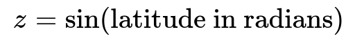
Longitude ranges from -180 to +180, and latitude ranges from -90 to +90. One way to manage their cyclical nature is to convert each angle into sine and cosine components:


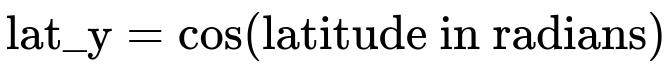
Each of these features (lon_x, lon_y, lat_x, lat_y) can then be fed into your model. The sin/cos transformation helps the model understand the wrap-around effect; for instance, -180 and +180 end up having nearly identical (sin, cos) pairs. You might then apply a standard scaler or min-max scaler to these new sin/cos features if numerical scaling is still desired.
Parameters explanation (inline text-based):
longitude in radians means longitude * (pi / 180).
latitude in radians means latitude * (pi / 180).
The sin function transforms the angle to a range in [-1, +1].
The cos function also transforms the angle to a range in [-1, +1].
The resulting (lon_x, lon_y) or (lat_x, lat_y) pairs preserve angular information.
Transforming into a 3D Spherical Representation
Another common strategy is to place each (latitude, longitude) pair on a 3D sphere, which can be viewed as embedding them into Cartesian coordinates (x, y, z). Specifically:


This representation preserves the global spherical structure of the Earth and ensures that points that are geographically close remain close in these 3D coordinates. Then you can choose to apply a further scaling mechanism (like standard scaling) if needed.
Using Local Projections
If your application involves a relatively small geographic area, you might sometimes adopt a local coordinate system (e.g., UTM projection or a simpler local projection like a meter-based or kilometer-based system). This local projection flattens the sphere locally, and you could then apply typical scaling approaches (like min-max scaling). This strategy avoids the complexities of global wrap-around because the region of interest is not large enough to encounter significant wrap-around errors.
Potential Pitfalls and Considerations
Handling the wrap-around effect:
Directly applying standard scaling to raw lat/long might cause discontinuities at boundaries like +180 and -180. This is a crucial reason for the sin/cos transformation or an alternative approach.
Handling polar regions:
Near the poles (latitude near +90 or -90), small differences in longitude might have less geographic significance in terms of actual distance. A spherical or 3D embedding approach handles this more gracefully than a naïve 2D scaling.
Geodesic distances:
If your model relies on real-world distances, consider the geometry of the Earth. Direct Euclidean distance in raw lat/long space does not represent actual “great-circle” distance. The 3D spherical embedding or explicit haversine formula is often necessary if precise distance calculations are needed.
Practical data range:
If the dataset covers a tiny region (e.g., a single city), standard scaling might be sufficient, but it is still not robust if your model depends on distances across the boundary of your coordinate range.
Follow-up Questions
How do you decide if it is better to use the 2D sin/cos approach or the 3D spherical representation?
It depends on the nature and scope of your problem. For a purely global application or when you want to preserve accurate distances across large portions of the globe, the 3D spherical approach is often superior because it naturally preserves proximity on the sphere. If your problem data is somewhat local or if you only care about general cyclical effects (like wrap-around), the sin/cos approach for both latitude and longitude can be simpler and still effective.
If you also need to compute or approximate distances between coordinates, a 3D representation or an explicit use of the haversine formula might be advisable. In many practical contexts, either representation is acceptable if the model is primarily using these variables as input features rather than directly computing distances among them.
How would you handle distance calculations once you have normalized coordinates?
If you have transformed your coordinates to a sin/cos 2D representation, using Euclidean distance on (lon_x, lon_y, lat_x, lat_y) does not strictly reflect great-circle distance. You might still need the haversine formula or a 3D Euclidean approach from the spherical coordinates if you want distances that mirror the Earth's surface. For an application that relies heavily on distance metrics (like nearest-neighbor queries, clustering, or any distance-based algorithm), using a geodesic-aware distance calculation is essential.
What if your data covers only a small region like a single city?
When focusing on a small region, the curvature of the Earth and the wrap-around at ±180 degrees might not be a significant factor. In such cases, you could project your lat/long to a planar coordinate system (for example, a UTM zone or a local projection used by GIS systems) and apply standard min-max or z-score normalization. This approach reduces the complexity of global coordinates. However, if there is a possibility that your data might expand to larger geographic coverage, planning for a robust approach (like spherical embedding) can save re-engineering effort later.
Could you use a standard scaler on raw lat/long if you only have local data?
Yes, if the area is small enough that you never cross the ±180-degree boundary and do not come near the poles, you can treat latitude and longitude as if they were effectively linear coordinates within that zone. A standard scaler would not break anything if the geographic coverage is small, and you do not require precise great-circle distances. However, keep in mind that this is a workaround that only applies in narrow contexts. For broader coverage or more accurate distance-based modeling, sin/cos transformations or 3D spherical representations are generally preferred.
Does the Earth's ellipsoidal shape affect these transformations?
Strictly speaking, yes. The Earth is not a perfect sphere; it is an oblate spheroid. Spherical approximations can introduce small errors when converting lat/long into x,y,z coordinates. For most machine learning tasks, especially if not operating at extremely high-precision geospatial scales, the spherical approximation is usually sufficient. If you require more geodetic accuracy, you can use more precise ellipsoidal formulas or local projections that match your region of interest closely.
Why does the 2D sin/cos transformation help with cyclical features?
Longitude is cyclical because -180 degrees is effectively the same place as +180 degrees. A similar concept applies in other cyclical contexts, such as hours on a clock (where 23 and 0 are just one hour apart). By converting angles to (sin, cos) pairs, the model sees that -180 and +180 have nearly identical values, capturing the cyclical wrap-around. Without this transformation, the model might learn an incorrect representation that places -180 and +180 too far apart in the feature space.
Example of Code for Sin/Cos Normalization
import numpy as np

def sin_cos_transform(lat, lon):
    """
    lat, lon are in degrees.
    Returns (lat_x, lat_y, lon_x, lon_y).
    """
    # Convert degrees to radians
    lat_rad = np.radians(lat)
    lon_rad = np.radians(lon)

    lat_x = np.sin(lat_rad)
    lat_y = np.cos(lat_rad)
    lon_x = np.sin(lon_rad)
    lon_y = np.cos(lon_rad)

    return lat_x, lat_y, lon_x, lon_y

# Example usage:
latitudes = [34.05, 36.12, 42.36, -23.55]
longitudes = [-118.24, -115.17, -71.06, -46.63]

for lat, lon in zip(latitudes, longitudes):
    lx, ly, ox, oy = sin_cos_transform(lat, lon)
    print(f"Lat: {lat}, Lon: {lon} -> (lat_x, lat_y, lon_x, lon_y) = ({lx:.3f}, {ly:.3f}, {ox:.3f}, {oy:.3f})")
You can further scale or feed these features into a deep learning model, tree-based model, or any other ML pipeline.
Below are additional follow-up questions
How does the type of machine learning model influence the choice of latitude/longitude normalization approach?
Answer (Detailed Reasoning):
Models sensitive to distance metrics (e.g., k-Nearest Neighbors, DBSCAN):
These models rely on pairwise distance calculations to group or classify points. A raw latitude/longitude input without proper handling of spherical geometry can lead to incorrect distance computations (especially across boundaries like ±180).
Why 3D spherical or sin/cos helps:
The 3D spherical approach preserves the actual closeness of points on the globe in Euclidean space.
The sin/cos transformation for each dimension (lat, lon) ensures cyclical continuity, but it’s not always a perfect reflection of great-circle distance unless you do more sophisticated distance measures.
Pitfall: If you simply apply standard scaling, distance-based algorithms may incorrectly interpret “close” points near ±180 degrees of longitude as far apart. This will degrade clustering or classification performance.
Neural networks (deep learning):
Neural networks can often learn nonlinear transformations, but providing them with already “angle-aware” features (like sin/cos or x,y,z on a sphere) can speed up training and improve performance.
Why sin/cos can be enough:
Many feed-forward or convolutional networks can handle these cyclical features quite well.
Pitfall: Relying solely on the network to learn wrap-around boundaries can require more training data and might produce suboptimal results compared to a well-designed feature representation.
Tree-based methods (e.g., Random Forest, Gradient Boosted Trees):
These do not rely on Euclidean distance in the feature space, so they may handle raw lat/long somewhat better than distance-based algorithms.
However: If lat = 179 and lat = -179 represent close points, trees might still have trouble discerning that those points are near each other.
Cyclical transform benefits:
Splitting on sin/cos or 3D coordinates can help trees recognize the wrap-around effect more consistently.
Linear models (e.g., Logistic Regression, Linear Regression):
Purely linear transformations of lat/long rarely capture the curved geometry of Earth.
Benefit of transformations:
Incorporating sin/cos or (x, y, z) can allow a linear model to approximate some nonlinear relationships in the geographic space.
Conclusion for model types:
Distance-based: 3D spherical or at least sin/cos is almost mandatory.
Neural networks: sin/cos or spherical can reduce the complexity of what the network must learn.
Tree-based: sin/cos or spherical can still help with boundary conditions.
Linear models: transformations are especially recommended so the model can better approximate relationships on a sphere.
What are the computational and performance trade-offs between using a 2D cyclical approach versus a 3D spherical embedding?
Answer (Detailed Reasoning):
Dimensionality:
2D cyclical (sin/cos for latitude and longitude): Results in four extra features (lat_x, lat_y, lon_x, lon_y) if you separate them out, or sometimes you might only transform longitude if you only care about one cyclical dimension.
3D spherical (x,y,z): Results in three features.
In terms of raw dimension count, 3D spherical can be simpler than four-dimensional sin/cos pairs.
Computational Cost:
Both transformations are straightforward to compute using sine, cosine, or a combination of them. The difference in cost per record is negligible, involving a few trigonometric function calls. In large-scale big-data pipelines, this difference is usually small compared to other processing tasks.
Interpretation and distance calculations:
2D cyclical:
If you measure Euclidean distance on (lat_x, lat_y, lon_x, lon_y), it’s not a direct measure of real-world distance. You would still need a specialized formula if you wanted true geographic distance.
This is, however, simpler to reason about for cyclical wrap-around specifically in each dimension.
3D spherical:
Points that are close on Earth’s surface generally remain close in 3D Euclidean space. A straightforward Euclidean distance in 3D approximates great-circle distance (assuming a spherical Earth).
It can be more intuitive for algorithms that use geometry or distance-based calculations.
Handling the Poles:
2D cyclical: The transformation captures each dimension’s periodic nature but does not automatically guarantee that latitudes near the poles are handled exactly like a sphere. However, the combination of lat_x, lat_y can reflect closeness near the poles.
3D spherical: By definition, it properly accounts for the spherical geometry. Poles end up as points (0, 0, ±1 in x,y,z) on the 3D sphere, which is more physically accurate.
Performance in ML tasks:
Typically, both approaches outperform raw lat/long in tasks that are sensitive to cyclical or spherical geometry.
The difference in performance between 2D cyclical and 3D spherical can depend on the dataset’s global coverage, the distribution of points, and the model type.
Can normalized latitude/longitude coordinates be combined with auxiliary geospatial data like altitude or population density?
Answer (Detailed Reasoning):
Adding altitude (or elevation):
If you have an altitude measurement, you can integrate it directly alongside your latitude and longitude transformations.
For the 3D spherical representation, you can add altitude by extending the radial distance from Earth’s center slightly. For example, ( r = R_{\text{Earth}} + \text{altitude} ), then compute ((x, y, z)) based on that new radius. However, you need to ensure the altitude is in the same units (e.g., meters) and is relatively small compared to Earth’s radius (~6371 km).
Pitfall: If you simply treat altitude as another feature, you must consider that near sea level vs. mountaintops might be relevant only if your model expects vertical distance to matter.
Population density or other geospatial features:
You can treat these features as standard numeric variables. Combine them with your transformed lat/long (be it sin/cos or x,y,z).
Scaling caution: If you use a standard scaler or min-max, do it either separately on each feature or as part of a pipeline that respects the nature of each feature.
Pitfall: In extremely large coverage areas, population density can vary widely. You may need to log-transform or apply specialized transformations.
Benefit of additional features:
The model can learn more context about each location, such as how heavily populated or how high above sea level it is. This can greatly improve predictions or classifications if these aspects are relevant.
How do we handle lat/long outliers or erroneous coordinates (e.g., lat = 200 degrees or lat = -370 degrees)?
Answer (Detailed Reasoning):
Detection of invalid ranges:
Valid latitude values must be between -90 and +90. Valid longitude values must be between -180 and +180.
If you see lat = 200, it’s outside the possible real-world range. This is likely a data quality issue or an encoding mistake.
Possible strategies:
Filtering/Removing records: If the fraction of invalid points is tiny, you might remove them from the dataset rather than attempt to “fix” them.
Clamping/Rolling: In some rare cases, if the data is systematically offset (e.g., a constant shift of +360 on longitude), you could re-map it by subtracting 360.
Imputation: If the missing/invalid coordinate is vital, you might impute (e.g., fill with a default “unknown” location or approximate with the mean location). But be aware this can degrade model performance if done incorrectly.
Pitfalls:
Blindly clamping (e.g., lat = min(max(lat, -90), 90)) can distort the data if you have many such outliers.
Mixed coordinate systems or mislabeled columns can cause bizarre lat/long. Always confirm your coordinate reference system (CRS).
Conclusion on outliers:
Clean and validate geospatial data before transformation to avoid introducing nonsensical sin/cos or 3D coordinates.
If you suspect systemic errors, investigate the data pipeline or device capturing lat/long (like a faulty GPS or incorrect format).
How do we interpret model predictions that use transformed latitude/longitude features?
Answer (Detailed Reasoning):
Challenge of indirect features:
Once lat/long are transformed (e.g., to sin/cos or 3D x,y,z), the features lose the direct interpretability of “degrees from the equator” or “degrees from the prime meridian.”
This can make explaining the model’s decisions more challenging because partial dependence plots or feature importances refer to lat_x, lat_y, lon_x, lon_y or x,y,z coordinates.
Reversibility of transformations:
You can convert (x, y, z) back to approximate lat/long by reversing the spherical formulas if you need to interpret or visualize a prediction in geographic terms.
If using sin/cos, you can do: [ \text{lon} = \arctan2(\text{lon_x}, \text{lon_y}), \quad \text{lat} = \arctan2(\text{lat_x}, \text{lat_y}) ] (Be mindful of quadrant issues and the domain/range of arctan2.)
Feature importance:
Tools like SHAP or permutation importance might show that lat_x, lat_y, lon_x, lon_y are collectively influential. But it won’t directly tell you “this area near 40°N is important.” You’ll have to interpret that cluster of features together.
Debugging and visualization:
If you want to see how the model might behave spatially, you could create a geographic grid, apply the transformation to each point, feed it into the model, and then map the outputs back to lat/long for visualization.
Pitfalls:
If you forget that your input to the model is cyclical or 3D, you might misinterpret linear relationships.
For example, you might see that high lat_x combined with certain lat_y leads to some classification, but converting that back to actual lat/long might reveal it’s near the poles.
Should we handle missing latitude/longitude values differently from how we typically handle missing numerical data?
Answer (Detailed Reasoning):
Uniqueness of lat/long data:
Latitude/longitude often serve as essential locational data. Dropping or mis-imputing them can be more impactful than, say, a missing continuous variable like “income.”
Options for dealing with missing geolocation:
Dropping rows: If location is critical and you have enough other data, you might remove any record missing lat/long. However, this might reduce your dataset size significantly if missingness is frequent.
Imputing with a sentinel value: You might assign a default location (like (0,0) near the Gulf of Guinea) or some special (lat_x=0, lat_y=0, lon_x=0, lon_y=0 in sin/cos space) to indicate “unknown.”
Pitfall: This can cause the model to interpret your sentinel location as a real geographic point. This might distort model outcomes if many unknowns cluster there.
Imputing with local mean or median: For instance, if data from the same user or region is partially known, you might approximate. However, lat/long is highly context-specific, so this approach can be very misleading unless you have strong domain rationale.
Model-based imputation: If you have correlated data (e.g., zip codes, region codes, or other location clues), you could train a model to predict lat/long for missing entries. This can be complex but may preserve more data.
Effect on transformations:
If lat/long is missing, you cannot compute sin/cos or x,y,z. You must either handle the missingness first or encode an “unknown” category if your model can handle partial missingness (like some tree-based implementations can with special indicators).
Edge cases:
If a large fraction of lat/long is missing, your geospatial analysis might be heavily compromised. Ensure you have a strategy that makes sense domain-wise.
If the dataset crosses the International Date Line, how do cyclical transformations handle that scenario?
Answer (Detailed Reasoning):
Longitude wrap-around at ±180°:
The International Date Line roughly follows 180° longitude, so crossing from +179.9° to -179.9° is effectively a small jump in geographic terms, but numerically it looks large if you store raw degrees.
sin/cos transformation:
(\sin(180°) \approx \sin(-180°)) and (\cos(180°) \approx \cos(-180°)).
This means those two points become nearly identical in the (sin, cos) space, correctly preserving the adjacency across the date line.
3D spherical approach:
Similarly, (x,y,z) for 179.9° and -179.9° are almost the same, again preserving adjacency.
Practical Pitfall in raw lat/long:
If you do not use a cyclical approach, standard scaling could treat +179.9 and -179.9 as being nearly 360° apart. A model might incorrectly interpret them as very far from each other.
This can severely degrade performance for any model relying on local neighborhoods.
Why cyclical transforms help so much here:
They mathematically unify those near ±180° points into nearly the same region of feature space, which matches their real-world geographic proximity.
Conclusion:
If your data is global and specifically crosses the date line, cyclical or spherical transformations are crucial to avoid incorrect boundary splits.
Can advanced dimensionality reduction techniques like PCA, t-SNE, or UMAP be applied to latitude/longitude data?
Answer (Detailed Reasoning):
Direct use on raw lat/long:
If you directly feed raw lat/long to PCA or t-SNE, you risk distorting global geometry because ±180 wrap-around is not recognized as close.
Additionally, PCA is linear and will not inherently capture spherical geometry. t-SNE and UMAP are nonlinear but can still be thrown off by wrap-around edges if lat/long is not transformed.
Benefit of first transforming to cyclical or spherical coordinates:
If you embed your points into a 3D sphere (x,y,z), then apply PCA or t-SNE:
The geometry is more consistent. You are letting the dimensionality reduction technique see the correct adjacency.
If you embed into sin/cos pairs, you can feed those into advanced methods. They will likely produce more meaningful clusters or 2D visualizations than raw lat/long alone.
Pitfalls in applying dimensionality reduction:
Overlapping or large-scale coverage: If your data is all over the planet, t-SNE or UMAP might group points in an abstract way that’s not purely geographical. They can group points by some manifold structure that might be only partially correlated with geography.
Computational complexity: t-SNE and UMAP can be computationally expensive if you have very large datasets.
Conclusion:
Yes, you can apply these techniques, but it’s often better to incorporate cyclical or spherical transformations first to respect Earth’s geometry.
Are there domain-specific transformations for maritime or aviation datasets?
Answer (Detailed Reasoning):
Maritime data specifics:
Maritime navigation often uses the concept of “nautical miles” and standard references to certain routes. The lat/long usage is the same globally, but there might be specialized projection systems or route-based data structures. For instance, you might see AIS (Automatic Identification System) data with frequent lat/long updates.
Potential transformations:
Spherical or sin/cos still help, especially for distance-based modeling.
Some maritime software tools adopt specialized projections near certain sea routes to minimize distortion.
Aviation data specifics:
Aviation often deals with flight levels (altitude), waypoints, or radial distances from VOR stations.
Coordinate references:
Pilots and flight systems rely on lat/long plus altitude, but also might consider local flight route coordinate systems.
The same basic geometry still applies. If analyzing flights worldwide, a 3D spherical representation plus altitude is very relevant.
Pitfalls:
Rapid changes in longitude crossing the date line is common in certain trans-Pacific routes. Failing to handle wrap-around can skew flight path analyses.
High-latitude routes near the poles (e.g., polar flights) require special attention to how lat/long is transformed.
Conclusion:
The fundamental transformations do not drastically change, but the domain might require adding other specialized features (e.g., altitude for aviation, water depth or port location for maritime).
Is there a risk of re-identification or data privacy leakage if lat/long are transformed or normalized?
Answer (Detailed Reasoning):
Reversibility of transformations:
If you use sin/cos or 3D spherical, it is still possible to invert these transformations back to approximate latitude and longitude. Therefore, a malicious actor could potentially re-identify specific locations if they gain access to the transformed data.
Even if you performed standard scaling on lat/long, a rough inverse transformation (given known approximate ranges) might reveal actual coordinates with some error margin.
Precision and granularity:
If you reduce the precision (e.g., rounding to the nearest city or some grid-based approach), it becomes harder to exactly re-identify individuals. However, you also lose some modeling fidelity.
Pitfall: Overly coarse rounding can degrade model performance on tasks where precise location matters.
Differential privacy or advanced anonymization:
In privacy-sensitive contexts, you might adopt more sophisticated methods, such as differential privacy, k-anonymity, or aggregated geohashes that can’t be trivially reversed.
These may reduce the risk of re-identification but come with a trade-off in predictive accuracy for location-based tasks.
Conclusion:
Merely transforming lat/long to cyclical or spherical coordinates does not guarantee privacy. If location privacy is critical, consider advanced anonymization or coarser data.
What if the application deals mostly with “bearing” or “direction” instead of absolute positions?
Answer (Detailed Reasoning):
Difference between “position” and “direction/bearing”:
Position: A lat/long coordinate on the Earth’s surface.
Bearing: The angle or direction from a reference point or your current heading in navigation (0° = North, 90° = East, etc.).
Cyclical nature of bearing:
Bearing is cyclical from 0° to 360° (or -180° to +180°). This is identical to the cyclical concept for longitude. If 360° is the same as 0°, you need cyclical handling (e.g., sin/cos).
Combining bearing with lat/long transformations:
You might have features for position (x,y,z or sin/cos lat, sin/cos lon) plus a separate cyclical transform for bearing (bearing_x = sin(bearing), bearing_y = cos(bearing)).
Pitfall:
Treating bearing as a standard numeric value can cause abrupt jumps near 0°/360°, misleading the model about the continuity in heading.
Conclusion:
If the problem is about direction or heading, use cyclical transformations for bearing just like you do for longitude or time-of-day.
How do we best validate that a chosen latitude/longitude transformation is working effectively?
Answer (Detailed Reasoning):
Quantitative checks:
Distance Preservation Tests: Compare known distances between pairs of points on Earth’s surface to the model’s implied distances in the transformed space (if you aim to preserve geometry). For example, pick a few pairs of well-known city coordinates, transform them, compute Euclidean distances, and see how they compare to great-circle distances.
Model Performance Metrics: If the transformation’s main purpose is to improve a predictive or classification model, measure the improvement (accuracy, RMSE, F1-score, etc.) after applying the transformation.
Visual inspections:
Plot your data on a 2D or 3D scatterplot (depending on your transform) and visually inspect if points near ±180° in longitude are indeed grouped closely.
For large coverage areas, a 3D spherical plot can confirm that continents or major regions are shaped correctly.
Edge/boundary cases:
Specifically check data near the International Date Line, near the poles, or any unusual boundary. If using cyclical transforms, see if those points are mapped logically close to each other in your transformed feature space.
Geospatial test using known neighborhoods:
If you have region or city labels, check that data points from the same region remain close in the transformed feature space. Conversely, points from different regions should remain relatively separate unless they’re geographically close.
Iterate and refine:
If you discover anomalies (e.g., polar data not grouping correctly, or crossing the date line not being recognized), you might switch from 2D cyclical to 3D spherical or apply local projections for smaller areas.
Conclusion:
Validation is both numerical (distance comparisons, model performance) and visual (plots, boundary checks). Ensure your transformations align well with the specific problem’s geographic scope and modeling goals.