ML Interview Q Series: How would you develop a system capable of detecting anomalies in streaming data in real time?

Mar 22, 2025

📚 Browse the full ML Interview series here.

Comprehensive Explanation

Real-time anomaly detection focuses on continuously monitoring incoming data and identifying unusual patterns or outliers as soon as they occur. This often involves ingesting data through a streaming pipeline, processing it to extract or transform features, applying a specialized algorithm to detect anomalies, and then delivering immediate notifications or corrective actions.

Connect with me on X (Twitter)

A common approach is to use incremental or online learning algorithms that update their internal parameters continuously, instead of requiring a full batch of data all at once. This can be particularly important in scenarios where data arrives rapidly and in large volumes. It is also crucial to keep track of concept drift, where the distribution of normal data evolves over time, and the definition of "anomaly" may shift.

Data preprocessing involves steps like normalization or scaling to ensure that data from different time intervals can be compared fairly. Sliding windows are often deployed to handle varying data rates. A sliding window can be of fixed size or a more adaptive scheme can be used to capture the most recent behavior.

After data ingestion and preprocessing, the anomaly detection algorithm determines whether a data point (or sequence) is deviant compared to what is considered normal. Traditional statistical methods might assume a particular data distribution, while more advanced techniques such as deep learning-based autoencoders, recurrent neural networks, or transformers handle non-linear relationships and time dependencies.

When using statistical approaches, one may assume the normal data distribution is Gaussian with a mean mu and a standard deviation sigma. Anomaly scores are computed based on how probable or improbable a new observation is, under the learned distribution. A deep learning strategy often relies on the reconstruction error of an autoencoder or the prediction error of an LSTM that models time-series data.

Below is a representative formula that might be central to a simple statistical anomaly detection method (like a Gaussian approach). The probability density for a data point x, assumed to be drawn from a normal distribution with parameters mu (mean) and sigma (standard deviation), can be written as:

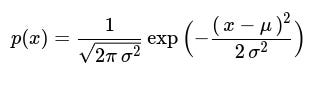
In this expression, x is considered anomalous if p(x) is sufficiently low, which indicates x is located in the extreme tails of the distribution. The parameters mu and sigma are updated incrementally using new data. mu can be updated with a running average, and sigma can be computed with a running variance. Over time, if the underlying data distribution changes, mu and sigma should reflect those changes.

Many deep learning algorithms for real-time anomaly detection use either a reconstruction error or a predictive error. For instance, an autoencoder tries to compress and then reconstruct input data. Points whose reconstruction error is unusually large may be deemed outliers:

where x is the original input and hat{x} is the reconstructed output from the autoencoder. In real-time scenarios, the autoencoder might be trained on a dataset assumed to be normal and then deployed to reconstruct new incoming data. If the model is re-trained or fine-tuned online, the parameters can adapt gradually to shifting normal behavior.

Practical Implementation Details

In practical streaming systems, data often arrives via message queues (like Kafka or RabbitMQ). A consumer service reads this data, preprocesses it, then feeds it into an anomaly detection model that updates or infers anomalies in real time. Latency requirements might dictate how complex your model can be. For instance, a simple statistical approach can be extremely fast, whereas a large deep learning model might introduce computational overhead.

The threshold for deciding what is an anomaly is normally set based on validation data or domain constraints. For example, if the domain is fraud detection in financial transactions, the threshold might be more aggressive to ensure suspicious transactions are flagged quickly, but at the cost of more false positives.

Below is a minimal example of a streaming anomaly detection loop using a deep learning model in PyTorch. This snippet shows a conceptual, simplified version of updating an autoencoder on the fly using a small batch of new streaming data:

import torch
import torch.nn as nn
import torch.optim as optim

class SimpleAutoencoder(nn.Module):
    def __init__(self, input_dim, latent_dim):
        super(SimpleAutoencoder, self).__init__()
        self.encoder = nn.Sequential(
            nn.Linear(input_dim, latent_dim),
            nn.ReLU()
        )
        self.decoder = nn.Sequential(
            nn.Linear(latent_dim, input_dim),
            nn.Sigmoid()
        )

    def forward(self, x):
        z = self.encoder(x)
        reconstructed = self.decoder(z)
        return reconstructed

# Instantiate the model and optimizer
model = SimpleAutoencoder(input_dim=10, latent_dim=3)
optimizer = optim.Adam(model.parameters(), lr=1e-3)
criterion = nn.MSELoss()

def update_autoencoder(new_data):
    # new_data is a torch.Tensor of shape (batch_size, input_dim)
    optimizer.zero_grad()
    reconstructed = model(new_data)
    loss = criterion(reconstructed, new_data)
    loss.backward()
    optimizer.step()
    return loss.item()

def infer_anomalies(new_data, threshold=0.01):
    model.eval()
    with torch.no_grad():
        reconstructed = model(new_data)
        reconstruction_error = (new_data - reconstructed).pow(2).mean(dim=1)
        # Compare reconstruction error to a threshold
        anomalies = reconstruction_error > threshold
    return anomalies

# Simulated streaming loop
import numpy as np

for step in range(100):
    # Generate synthetic data batch
    data_batch = torch.FloatTensor(np.random.rand(4, 10))
    # Update model
    training_loss = update_autoencoder(data_batch)
    # Detect anomalies
    anomalies_detected = infer_anomalies(data_batch)
    # Real systems might log or publish these anomalies
    print(f"Step {step}, Training Loss: {training_loss}, Anomalies: {anomalies_detected}")

This simple code demonstrates partial online updates to a model and inference for anomalies in real time. The threshold for anomalies in infer_anomalies is just a toy example. In practice, it can be dynamically estimated using a rolling quantile of errors or domain-specific guidelines.

Key Considerations

Real-time anomaly detection is more than just choosing an algorithm. It involves designing a robust data pipeline, setting thresholds or confidence intervals, implementing a monitoring and alerting system, and planning how to respond when anomalies are flagged. It also often requires a feedback loop to label flagged anomalies. This new information can be used to refine the model incrementally or offline.

Handling concept drift is especially important. If the environment changes significantly, old data might no longer represent current conditions. Techniques like windowing and forgetting factors help models “forget” outdated patterns. Some advanced systems measure how dramatically data statistics change over time and automatically trigger model updates or re-training.

How to Handle Concept Drift

Concept drift occurs when the statistical distribution of the incoming data changes. In real-time scenarios, it is beneficial to maintain a running average for the mean and standard deviation, or use models capable of partial fit. Another strategy is to keep a limited window of most recent data for training. If the environment changes slowly, small incremental updates suffice. If it changes abruptly, a more thorough re-initialization or heavier re-training might be necessary.

Choosing a Threshold for Anomaly Detection

In practice, thresholds can be selected by analyzing historical data or by domain knowledge. If you have some labeled data indicating what normal and anomalous points are, you can set the threshold so that the false positive rate remains below a certain level. Alternatively, you could set a threshold based on statistical quantiles in a validation period or choose an empirical percentile of reconstruction errors.

Evaluating Real-Time Anomaly Detection

Evaluation typically uses precision, recall, F1 score, or area under precision-recall curves, if ground-truth labels are available. However, obtaining real-time labeled data can be challenging. Sometimes evaluation is performed retrospectively. Another approach is to run the system in parallel with an existing anomaly detection pipeline until confidence is established in the new method’s performance.

Possible Follow-Up Questions

How do you integrate real-time anomaly detection with alerting systems?

One strategy is to have a messaging or event pipeline that triggers alerts when anomalies exceed certain thresholds. Alerts can go to dashboards, emails, or on-call personnel. To avoid alert fatigue, one must carefully tune thresholds to reduce false positives and employ aggregation logic, so multiple anomalies in a short time frame trigger a single actionable alert.

What if the data is heavily imbalanced?

Real-time streams often contain far more “normal” samples than “abnormal.” Certain anomaly detection methods that assume balanced data may underperform. Techniques like oversampling of historical anomalous cases or specialized loss functions for imbalanced data can help. For unsupervised models, dealing with imbalance might require refined thresholding or adding additional features that characterize normality more precisely.

Can we use unsupervised methods if we have limited anomaly labels?

Yes. Unsupervised anomaly detection (like autoencoder-based reconstruction error or clustering-based approaches) does not rely on labeled anomalies. It learns what normal data looks like and flags points that deviate from this learned profile. If minimal labels are available, semi-supervised approaches can incorporate that information to improve the model’s performance.

How do you select a window size in a streaming environment?

Window size decisions depend on the stationarity of the data and how quickly you expect the distribution to change. A shorter window updates model parameters rapidly but may cause volatility and higher false positives. A longer window results in smoother, more stable estimates but may lag in detecting sudden shifts. It can be beneficial to experiment with different window lengths or use an adaptive windowing method based on the rate of concept drift.

How do you ensure scalability in real-time anomaly detection?

Scalability can be achieved by distributing the load across multiple processing nodes or microservices. For example, data might be partitioned by key (e.g., sensor ID or user ID), and each partition is processed independently with its own anomaly detection model. This can be scaled horizontally. For computationally heavier models, it can help to offload model inference to GPUs or specialized hardware, or adopt approximate methods (e.g., random projection or sampling) that reduce complexity while maintaining good performance.

Below are additional follow-up questions

How would you handle real-time anomaly detection if the data is non-stationary and exhibits random bursts of outliers that might actually be part of normal system behavior?

When data is non-stationary, the distribution and characteristics of “normal” behavior can shift over time. This can lead to false alarms if your model has been trained on an older distribution that no longer accurately represents the system. One approach to mitigate this is by employing rolling windows and incremental updates. A rolling window allows the model to adapt only to the most recent data, gradually forgetting old patterns that may no longer apply. However, if the system experiences random bursts of outliers that are actually normal in certain contexts (for example, retail data spikes during holiday seasons), an overly sensitive model might trigger false alerts.

A practical mitigation strategy involves maintaining a buffer of known “normal burst” scenarios. When a burst is detected, compare the incoming data to historical bursts of similar magnitude, duration, or pattern. If they match, the model treats it as a normal (albeit extreme) occurrence. If it diverges significantly from known patterns, the system flags it as a potential anomaly.