ML Interview Q Series: How would you perform gradient boosting using decision trees?

📚 Browse the full ML Interview series here.

Comprehensive Explanation

Gradient boosting with decision trees is an iterative technique that builds an ensemble of weak learners (often small decision trees). Each new tree attempts to correct the errors made by the previous ensemble, typically by fitting to the negative gradient of the loss with respect to the model’s predictions. Through repeated addition of these weak learners, the overall model becomes more accurate.

One way to see gradient boosting is as an additive model that continuously refines its predictions by focusing on the residual errors (or the negative gradient of a loss function) left by preceding trees. At each iteration, the algorithm fits a new tree to these residuals, scales it by a learning rate, and updates the overall ensemble.

Below is the core update formula (in large format as per instructions). We define F as our ensemble model, m as the iteration index, and h_m as the new weak learner (tree) trained at iteration m:

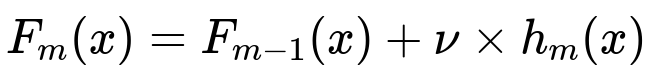
Here, F_{m-1}(x) is the model from the previous iteration, h_{m}(x) is the newly fitted tree at the m-th step, and \nu is the learning rate (a small scalar typically in the range 0.01 to 0.3). After fitting the new tree h_{m}(x), the ensemble F_{m}(x) is updated by adding the scaled version of h_{m}(x) to the previous model’s output.

Step-by-Step Logic

Initialization Typically, you start by taking F_{0}(x) as the model that predicts the average of the target values for regression or the log-odds for classification. This acts as the initial guess.

Compute Residuals (or Negative Gradients) For every training instance, compute the gradient of the loss with respect to the predictions of the current ensemble. In simpler contexts (like least squares regression), these gradients reduce to raw residuals. For other differentiable loss functions, such as cross-entropy, we calculate the negative partial derivative of the loss with respect to the model’s outputs.

Train a Weak Learner Use these gradients (pseudo-residuals) as the target labels to train a new decision tree. The idea is that this tree will learn how to correct or reduce the current errors.

Find Optimal Coefficients (Line Search) After training the tree, one can optionally perform a line search to find the best scalar multiplier for each leaf (or a single multiplier for the entire tree) that best minimizes the original loss when added to the current ensemble.

Add the Scaled Tree to the Ensemble Scale the tree’s outputs by the learning rate and add it to the existing model. This finalizes the update step:

F_{m}(x) = F_{m-1}(x) + scaled_tree.

Important Hyperparameters and Considerations

Learning Rate (nu) The learning rate controls the magnitude of the update at each iteration. A smaller learning rate makes the training more robust to overfitting but typically requires more iterations (trees). A larger rate reduces the number of trees needed but may lead to overfitting if it is too large.

Number of Trees More trees typically yield a lower training error, but can risk overfitting. Methods like early stopping, where you track validation error and stop when it stops decreasing, help avoid overfitting.

Tree Depth Shorter (shallower) trees can serve as weak learners and reduce overfitting, but might underfit if the tree depth is too small. In practice, a maximum depth of 3–8 is common for gradient-boosted trees.

Subsampling Some implementations use random subsampling of the data for each new tree (similar to stochastic gradient descent). This approach can speed up training and combat overfitting by injecting randomness.

Regularization Techniques like L1/L2 regularization on leaf weights, limiting tree complexity, or using constraints on leaf node outputs are all methods to reduce overfitting. Common frameworks (like XGBoost, LightGBM, CatBoost) include advanced regularization terms to better control complexity.

Practical Python Example

Below is a simplified example of using gradient boosting with decision trees in Python, illustrating how you might train a gradient-boosted model with scikit-learn:

from sklearn.ensemble import GradientBoostingRegressor
from sklearn.datasets import make_regression
from sklearn.model_selection import train_test_split
import numpy as np

# Generate synthetic data
X, y = make_regression(n_samples=1000, n_features=10, noise=10, random_state=42)

# Split into train and test
X_train, X_test, y_train, y_test = train_test_split(X, y, test_size=0.2, random_state=42)

# Create a Gradient Boosting regressor
gbr_model = GradientBoostingRegressor(
    n_estimators=100,
    learning_rate=0.1,
    max_depth=3,
    subsample=0.8,
    random_state=42
)

# Train the model
gbr_model.fit(X_train, y_train)

# Evaluate on test set
test_score = gbr_model.score(X_test, y_test)
print(f"Test R^2 score: {test_score:.4f}")

This code uses GradientBoostingRegressor from scikit-learn. Under the hood, it follows the gradient boosting procedure: building trees one at a time, each fitting to the negative gradient of the loss with respect to the current model predictions.

Potential Follow-Up Questions

What is the role of the negative gradient in gradient boosting?

The negative gradient of the loss function, computed with respect to the model's predictions, determines the direction in which we need to adjust our model to improve it. In gradient boosting, this negative gradient is treated as the target for the next weak learner. For example, in a mean-squared error context, the negative gradient corresponds directly to residuals (actual - predicted). In a logistic regression context, these gradients involve the derivatives of the logistic loss. This approach allows gradient boosting to be applied to various differentiable loss functions, making it very general and powerful.

How do we control overfitting in gradient boosting?

Overfitting can occur if the ensemble grows too complex. Key methods to control it:

• Limit the maximum depth of each tree to keep them weak and reduce variance. • Use a smaller learning rate so that each step is conservative, though it will require more trees. • Incorporate regularization techniques such as shrinking leaf weights or adding L1/L2 penalties. • Employ subsampling of rows (and sometimes columns) to introduce randomness and reduce correlation between trees (stochastic gradient boosting). • Monitor validation error and stop early when performance no longer improves.

Why do gradient-boosted decision trees often outperform random forests?

Random forests average predictions from fully grown, decorrelated trees, which lowers variance but can still leave some bias in the model. Gradient boosting, by contrast, builds an additive model in a forward stage-wise fashion, which directly tackles the residual errors of prior trees. This often leads to lower bias because each new tree corrects the mistakes made so far. However, gradient-boosted methods tend to be more sensitive to hyperparameter settings and can overfit if not carefully tuned (learning rate, tree depth, number of trees, etc.).

How is gradient boosting adapted for classification problems?

For classification, gradient boosting commonly uses a differentiable loss like log-loss (binary cross-entropy). The negative gradient in that case becomes a function of probabilities (or log-odds). Each tree is fit to these gradient values, effectively learning which samples the current model is classifying with large error. After building each tree, the ensemble is updated in the direction that reduces the classification error in a gradient descent manner. For multi-class settings, frameworks apply this logic to each class dimension or use specialized algorithms (e.g., one-vs-all or one-vs-rest strategies).

What are some practical implementation considerations for gradient boosting at scale?

• Efficient Data Structures: Libraries like XGBoost use advanced data structures (e.g., quantile-based histograms) for fast split finding. • Parallelization: Training many trees can be parallelized, though gradient boosting is more sequential than random forests, so you may parallelize within each iteration by distributing work across multiple cores or machines. • Memory Usage: For large datasets, consider out-of-core (streaming) approaches or distributed frameworks to avoid memory bottlenecks. • Hyperparameter Tuning: Automated methods (Bayesian optimization, grid search, random search) can systematically find the best hyperparameters. This is especially relevant at scale where multiple runs can be time-consuming.

How do popular libraries like XGBoost or LightGBM optimize gradient boosting?

• XGBoost: Improves gradient boosting primarily with sophisticated tree split algorithms, block-based parallelization, out-of-core computation, and regularization techniques. • LightGBM: Uses gradient-based one-side sampling (GOSS) and exclusive feature bundling (EFB) to drastically reduce computational cost and memory usage, enabling it to handle huge datasets with many features. • CatBoost: Offers specialized methods for dealing with categorical variables and employs ordered boosting to reduce prediction shift.

Each library implements clever strategies to build trees faster and with better resource efficiency, while also adding specialized regularization and techniques to handle real-world data challenges.

Could you show the difference between gradient boosting and AdaBoost?

AdaBoost also builds an ensemble of weak learners but focuses on re-weighting misclassified examples rather than fitting to the negative gradient of a loss. Gradient boosting generalizes this idea to arbitrary differentiable loss functions and computes pseudo-residuals as targets. AdaBoost can be seen as a special case of gradient boosting under the exponential loss. The greater flexibility of gradient boosting with different loss functions typically yields broader applicability and potentially higher accuracy.

How do you prevent your trees in gradient boosting from simply memorizing outliers?

Outliers can exert a strong influence on the loss and cause large gradients. Key strategies:

• Use robust loss functions (like Huber loss) which reduce the effect of large residuals. • Cap the maximum number of leaf nodes or limit the leaf node output to prevent extreme predictions. • Employ regularization (shrinkage, L1/L2 penalties) to reduce overfitting. • Use early stopping to halt training before the model overfits heavily to extreme values.

By carefully tuning these parameters and using robust approaches, you can make the training less sensitive to outliers while still benefiting from the iterative improvements of gradient boosting.