
ML Interview Q Series: How would you explain loan rejections from a binary classifier without access to feature weights?

📚 Browse the full ML Interview series here.
Comprehensive Explanation
One effective way to address this scenario is through post-hoc interpretability methods. Because direct feature weights are unavailable, the key idea is to use techniques that approximate or probe the model’s behavior around a given instance to uncover which inputs contributed most strongly to the classification. Methods such as LIME (Local Interpretable Model-agnostic Explanations) and SHAP (SHapley Additive exPlanations) are useful for deriving local explanations of complex models, even if we do not have direct access to their internal parameters.
LIME approximates the local decision boundary of the model around a specific instance by generating perturbed samples and observing the model’s outputs for those perturbations. SHAP is grounded in cooperative game theory and calculates how much each feature contributed to pushing the prediction away from a baseline prediction value for a particular instance. This is done even if the original model is a black box, because SHAP only needs to query the model’s outputs for various input combinations.
Because we are dealing with loan applicants who are rejected, the main idea is to select a technique that can generate local feature attributions. That output, once generated, can be mapped to the original set of features (for example, credit score, income level, employment status) and used to indicate which ones most strongly influenced the decision toward rejection. This allows the financial institution to provide the applicant with high-level insights such as: “Your credit score was significantly below our threshold,” or “Your current debt-to-income ratio is too high,” based on the features that caused the model to lean towards rejection.
When providing such reasons, it is critical to translate the post-hoc interpretability output into user-friendly statements. In a regulatory context like lending, these user-friendly statements should be factual, relevant, and actionable. For instance, stating that “Your recent late payments were a strong factor” is more transparent and useful than purely numerical or abstract references to model internals.
In many real-world systems, local interpretability methods are used to create “reason codes.” These reason codes indicate the top few features that contributed most to the adverse decision. Systems can be designed to translate these features into an explanation that addresses the applicant, ensuring compliance with regulations and maintaining transparency.
One of the core mathematical underpinnings when generating local explanations using SHAP involves the Shapley value formula from cooperative game theory:
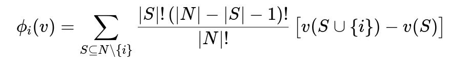
Where N is the set of all features, S is a subset of features that does not include the i-th feature, v(S) represents the prediction when only features in S are present, and |S|! * (|N|-|S|-1)! / |N|! is a combinatorial term reflecting the idea of treating each feature's contribution in all possible permutations. Essentially, the Shapley value for a feature i is an average of the marginal contributions of including that feature across all subsets of other features.
Translating these Shapley values into a rejection reason means identifying which features have the largest negative contribution to the applicant’s final score or decision. For example, if a low income variable had the highest negative SHAP value, that suggests the low income was a strong driver towards rejection.
Example Code Snippet
import shap
import numpy as np
import xgboost as xgb

# Suppose you have a trained XGBoost model:
model = xgb.XGBClassifier()
# model.fit(X_train, y_train)  # Already trained somewhere else

# Create a SHAP explainer for the model
explainer = shap.Explainer(model, X_train)

# Select one applicant instance who was rejected
applicant = X_test[0]

# Get SHAP values for that single instance
shap_values = explainer(applicant)

# Convert SHAP values into a readable plot or numeric array
shap.plots.waterfall(shap_values[0])

# The features with the greatest negative SHAP values
# can be highlighted as reasons for rejection.
In a production system, you might convert these top negative features into user-friendly textual explanations that convey a clear rationale, like “Your income level is below the acceptable threshold,” or “Your existing outstanding debt is too high relative to your total income.”
Follow-up Questions
How would you handle scenarios where the model is extremely complex or expensive to query repeatedly?
In some cases, repeatedly querying the model (as techniques like LIME or SHAP do) can be computationally expensive if the model is very large. One approach is to use more efficient approximation-based methods for local interpretation. You could train a simpler surrogate model (like a small decision tree) specifically around each applicant’s neighborhood. This reduces the number of queries needed and can still provide decent local explanations. However, it comes at the cost of some accuracy in pinpointing the exact contributions. Another tactic might be to sample fewer perturbations in LIME or approximate Shapley values using a smaller subset of the feature subsets, thereby reducing computational overhead while still retaining interpretability.
What if the same feature contributions appear contradictory for different applicants?
It is possible for different applicants with similar features to receive different rejection reasons if the model interacts with other features in a non-linear manner. In such cases, local interpretation is essential because a global rule might not exist. The best practice is to compute individual explanations for each rejected applicant. If contradictory or confusing explanations arise, it may signal that the model’s decision boundary is particularly sensitive or that there could be data quality issues. Exploring partial dependence plots or investigating higher-order interactions can clarify these differences.
Is there a risk of exposing proprietary model information by providing too many details?
Yes, providing extremely detailed feature attributions can inadvertently disclose sensitive information about the model or about how certain features weigh on decisions. To address this, explanations should typically be limited to the top few contributing factors, and you might obfuscate exact numeric contributions if necessary. The primary intent in regulatory or consumer-facing environments is to offer clear, actionable reasons rather than to reveal every subtle nuance of the model. Striking a balance between transparency and privacy is crucial.
Could post-hoc explanations lead to gaming the system?
There is a concern that if you reveal too much about how the model makes decisions, applicants might adjust their data or behavior in superficial ways just to pass the threshold. This “gaming” risk is a typical challenge in interpretability. Companies may mitigate this by focusing on stable and robust features that truly reflect creditworthiness, or by regularly updating their models so any “gaming” tactic becomes less effective over time. Additionally, good feature engineering and data validation can detect unnatural changes or anomalies in the input data.
How do you validate the correctness of these local explanations?
Ensuring the fidelity of local explanations requires cross-checking several metrics. One approach is to measure how closely the surrogate explanations (e.g., in LIME) match the actual model predictions within the local neighborhood. For SHAP, you can evaluate whether the Shapley values summation aligns with the difference between the predicted output and the baseline output. Another sanity check is to tweak a top-feature identified in the explanation and observe whether the model prediction changes in the expected manner (for instance, artificially increase a rejected applicant’s “income” feature in the input sample to see if the model would flip to approval).
How might the absence of feature weights in the original model limit your explanation strategies?
Not having direct feature weights restricts you from making immediate global statements about feature importance. You are confined to local or sample-specific interpretations. While this is not necessarily a bad thing—local interpretability can be more precise for individual decisions—it makes it more difficult to characterize overall feature contribution patterns across the entire dataset. In high-stakes settings like lending, local explanations are often sufficient for regulatory compliance as long as they clarify the specific decision at hand.
How can we ensure fairness and non-discrimination when providing reasons for rejection?
Fairness audits and bias checks should be conducted both during model training and post-deployment. Even if reasons are provided locally through an explanation tool, it is important to track whether protected groups (such as by race, gender, etc.) might be disproportionately impacted. Checking the distribution of rejection reasons across different groups can reveal if the model—or the data feeding into it—contains underlying biases. Remediating these biases may involve re-sampling, re-weighting, or making changes to the features used by the model. Providing a reason does not excuse the institution from ensuring that their decision-making process is fundamentally fair and legal.
These measures—together with robust post-hoc interpretability methods—help companies comply with regulations that require them to provide meaningful reasons for adverse decisions, despite not having direct access to feature weights within the black-box model.
Below are additional follow-up questions
What if the data contains highly abstract or engineered features that are not intuitively understandable to a layperson, such as latent embeddings?
When dealing with features that are naturally opaque (for example, embeddings learned from deep neural networks or other dimensionality-reduction processes), the primary challenge is to provide a reason for rejection in terms that a user can easily comprehend. Post-hoc explanation tools might identify that a certain embedding dimension contributes significantly to the model’s output, yet that dimension does not map cleanly to a real-world concept.
A possible strategy is to trace the latent features back to more interpretable precursors. For instance, if an embedding is derived from a user’s payment history or transaction details, you might cluster the dimensions in that embedding to see whether they align with known behavioral patterns. A local explanation method might show that these embedded factors correlate with tardy payments or unusual expense patterns. Translating that into a user-facing reason could become: “You often had payments that were more than 30 days late within the past year.”
Pitfalls:
Over-simplification could happen if you reduce a complex high-dimensional space to a few textual labels. This risks giving incomplete or misleading explanations.
Latent embeddings might inadvertently capture sensitive information (e.g., race or marital status) through correlations. You need to audit these representations carefully to ensure fairness and legal compliance.
How should we proceed if multiple features are highly correlated, making it unclear which actually caused the negative decision?
When features are correlated, standard post-hoc approaches can create overlapping attributions. SHAP, for example, assumes feature independence to compute contributions, though advanced variants try to correct for correlations. If two features (like debt-to-income ratio and total monthly expenses) are strongly correlated, they might both receive large negative contributions in a rejection scenario, leaving you uncertain which truly triggered the decline.
In practice, you can analyze feature interaction effects. Partial dependence or interaction plots can help reveal whether a single feature dominates or if the combination truly drives the rejection. You might also look at domain-specific logic to see which is more critical for underwriting decisions.
Pitfalls:
Overcounting or undercounting certain features in explanations, which can lead to confusion for applicants.
If you strip correlated features out of your model to simplify explanations, you may degrade performance. Balancing interpretability against predictive power is a real-world challenge.
How can we ensure regulatory compliance (e.g., GDPR’s “right to explanation”) without overwhelming applicants with technical jargon?
Regulations such as GDPR stipulate that individuals have a right to a meaningful explanation when they are subject to automated decision-making. Providing purely technical details or model internals could satisfy transparency from a developer’s point of view but might baffle the applicant and fail the requirement of “meaningful” explanation.
A practical approach is to build layered explanations:
A high-level summary: “Your application was rejected because your financial indicators did not meet our threshold.”
A mid-level explanation: “Your credit score was lower than typical approved applicants, and your total debt ratio was above our acceptable range.”
A deeper technical layer: available upon request, which includes more specific details about how the model arrived at the decision.
Pitfalls:
Over-informing applicants with too much complex detail might lead to confusion or cause them to draw erroneous conclusions.
Under-informing them could violate the spirit of the law or result in regulatory scrutiny.
How do we maintain consistent explanations over time when the model is retrained or updated frequently?
Models used in loan approval systems often undergo periodic retraining on more recent data to adapt to new patterns (for instance, changes in economic indicators). These updates might alter how feature importance is distributed, thus changing the post-hoc explanations.
You can keep a versioned history of models and corresponding explanation frameworks. Each time a model is deployed, you store a snapshot of the interpretability artifacts. This ensures that if an applicant challenges a past decision, you can reproduce the exact environment and show what the explanation would have been at that time.
Pitfalls:
A mismatch could occur between the version of the model that made the decision and the version used for generating explanations.
Frequent updates might create an inconsistent applicant experience, where two people with similar profiles receive different or even contradictory reason codes.
If the model is trained on incomplete or noisy data, how do we account for potential errors in providing reasons for rejection?
Data quality is critical for both predictive accuracy and reliable explanations. If training data is noisy—missing or misreported values—a perfectly functioning interpretability method might still produce misleading reason codes.
One mitigation strategy is to implement data validation checks before training the model and again before generating explanations. If key features show unusual distributions or questionable patterns, you might incorporate uncertainty estimates into your explanations. For example, “Our records indicate your monthly income is significantly lower than average, but we observed inconsistencies in your reported data. Please verify these details.”
Pitfalls:
Over-reliance on unvalidated data can lead to spurious or incorrect reasons for rejection.
If data errors disproportionately affect certain groups, it can amplify fairness concerns.
What if certain features behind the decision cannot be disclosed for legal or privacy reasons?
Certain regulated domains or proprietary data sources might prevent you from revealing exactly which inputs are used in the model. For example, an institution might have anti-fraud algorithms that hinge on confidential behavioral signals.
In such cases, you can provide partial or aggregated explanations. Instead of naming the exact feature (e.g., “Suspicious Transaction Pattern #435”), you might classify it more generally as “Transaction activity patterns flagged as high risk.” This maintains some level of transparency without revealing sensitive details that could compromise security or violate third-party data agreements.
Pitfalls:
Striking a balance between satisfying transparency requirements and keeping proprietary or sensitive information confidential.
Potential user mistrust if you are too vague: “Our system flagged your application as high risk due to proprietary indicators.”
How do we handle scenarios where different stakeholders require different forms of explanation (e.g., auditors vs. applicants vs. internal teams)?
Different stakeholders have different technical backgrounds and objectives. Auditors may want detailed logs and compliance documentation, while applicants simply want to understand why they were rejected, and internal teams may want actionable insights to refine the business logic.
One strategy is to build a multi-layer explanation framework. You can store comprehensive logs (SHAP value breakdowns, random sample queries from LIME, or rule-based surrogate trees) for auditors or technical teams. Meanwhile, applicants would see a simpler, plain-language reason code system. Internal stakeholders, like risk analysts, might need partial but more data-driven detail that is above the applicant’s summary level but below full raw logs.
Pitfalls:
Maintaining multiple explanation layers can be complex and prone to versioning errors. If they diverge, it can lead to inconsistencies.
Overly technical explanations can frustrate applicants; oversimplified ones might not satisfy auditors.
How do we handle large-scale deployments with millions of applicants while still providing individualized explanations?
Generating local explanations for every single applicant can be computationally heavy, especially if you must sample multiple perturbed inputs for each explanation. For large-scale operations, you can adopt a hybrid approach. For common applicant profiles, you may cluster them and pre-generate typical explanations that apply to each cluster. For edge or borderline cases, you can still compute a fresh local explanation on-demand.
Pitfalls:
Using pre-generated explanations for clusters might hide individual nuances, leading to misinterpretation if an applicant’s data within a cluster is slightly different.
On-demand methods might create latency issues in real-time loan decision systems if the interpretability technique is too slow.
In what ways might the model’s architectural constraints or feature engineering process influence the explanation method used?
Some models or features are naturally more amenable to certain explanation techniques. For instance, tree-based models can leverage specialized methods (like TreeSHAP) that are faster and more accurate for hierarchical splits, while neural networks might require more generalized methods.
If your data pipeline involves heavy feature transformations (like polynomial features, logs, or binning), you’ll need to ensure that the explanation method references the original raw features in a meaningful way. Failing to do so might lead to confusion: an explanation method might surface “x1_squared” as a top factor, but the applicant only recognizes their raw “annual_income.”
Pitfalls:
Explanations that focus on engineered features could be meaningless to end-users if not mapped back to something interpretable.
Certain black-box ensembling techniques might complicate feature attribution, requiring specialized or approximate solutions for valid explanations.