ML Interview Q Series: How would you contrast Naive Bayes against Logistic Regression when handling classification tasks?

📚 Browse the full ML Interview series here.

Comprehensive Explanation

Naive Bayes and Logistic Regression are both widely used techniques for solving classification problems, yet they rely on different assumptions and theoretical foundations. Understanding their distinctions is valuable because it helps one choose the model that best fits a particular problem scenario.

Naive Bayes

Naive Bayes applies Bayes’ Theorem with the “naive” assumption that the features are conditionally independent given the class label. Despite this strong assumption, Naive Bayes often performs surprisingly well in many real-world problems, especially those involving text classification with high-dimensional feature spaces such as spam filtering.

The core idea can be summarized by expressing the posterior probability of a class y given features x1, x2, ..., xn as proportional to the prior times the likelihood of the features:

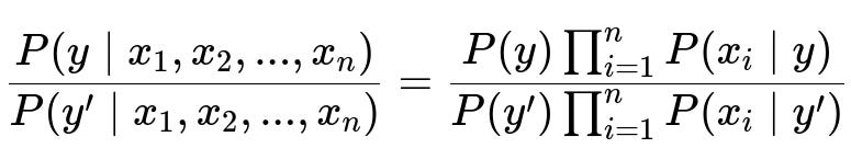
In the above expression, P(y | x1, x2, ..., xn) represents the posterior probability of class y given the features x1 through xn. P(y) is the prior probability of class y based on the training data. The term P(x_i | y) is the likelihood of feature xi given the class y. The strong conditional independence assumption simplifies the joint probability of x1, x2, ..., xn given y into a product of individual probabilities.

In practice, various versions of Naive Bayes exist (e.g., Gaussian, Multinomial, Bernoulli), each differing in how P(x_i | y) is modeled. For instance, Multinomial Naive Bayes is a common choice for text classification, where feature counts or term frequencies are typical features.

Logistic Regression

Logistic Regression, despite its name, is essentially a linear classifier in log-odds space. It models the logit function of the probability of belonging to a particular class, typically denoted as the probability of y=1 given the feature vector x. It uses a linear combination of the input features within the logistic (sigmoid) function. The sigmoid function is often denoted as:

Here, x is the vector of features (including a bias term), and theta is the vector of parameters. The output of sigma(theta^T x) is a value in the range (0,1), which can be interpreted as the probability of class y=1. The logistic loss (also called the cross-entropy loss) is typically minimized to find the best parameters theta.

Logistic Regression does not rely on the naive conditional independence assumption. Instead, it attempts to directly estimate the probability that y=1 for any given input x by finding a linear decision boundary in feature space (transformed by the sigmoid). Regularization (L2 or L1) is often used to prevent overfitting, especially when the number of features is large.

Key Contrasts

Interpretability. Naive Bayes, through the Bayes’ Theorem perspective, provides a direct explanation of how prior probabilities and feature likelihoods combine. Logistic Regression offers interpretability in terms of learned weights that show how each feature contributes linearly to the log-odds.

Statistical Assumptions. Naive Bayes assumes conditional independence between features given the class. Logistic Regression does not impose this assumption but instead uses a logistic function over a linear combination of features.

Performance. In practice, Naive Bayes can be quick to train and effective in high-dimensional, sparse data settings. Logistic Regression usually benefits from more training data and can often provide better probabilistic calibration.

Feature Correlation. Logistic Regression can handle correlated features better, while Naive Bayes may double-count the effects of correlated features due to its independence assumption, possibly deteriorating performance in such scenarios.

Parameter Estimation. Naive Bayes uses counts (or sums) to compute probabilities of features given classes. Logistic Regression uses gradient-based optimization to minimize the logistic (cross-entropy) loss function.

When data is truly high dimensional and somewhat sparse (e.g., text classification) and you want a quick baseline, Naive Bayes tends to work very well. When you have enough data and want a more refined approach without strong independence assumptions, Logistic Regression is often more flexible.

Follow-up Questions

What happens if some features are highly correlated in Naive Bayes?

Naive Bayes explicitly assumes that all features are conditionally independent given the class. When some features are highly correlated, the model effectively double-counts (or more) the effect of those correlated features. This can lead to overconfident predictions or skewed class probabilities. The severity of this overconfidence depends on how strongly the features are correlated and how many such correlated groups exist. In some cases, the model can still perform adequately, but in others, performance can degrade significantly.

One practical workaround is to remove or combine correlated features prior to training. Another approach is to use more sophisticated Bayesian networks that relax the naive independence assumption, but these models can be more complex and less computationally efficient.

When might Logistic Regression fail compared to Naive Bayes?

Logistic Regression might fail or underperform when the dataset is relatively small, the features are numerous, and the problem is high-dimensional. Logistic Regression typically requires a sufficient amount of data to estimate parameters reliably. If you have thousands of features but only a few hundred samples, overfitting can easily occur unless strong regularization is applied. Even then, performance might not be as good as a Naive Bayes model that gracefully handles sparse, high-dimensional data.

Additionally, if your data naturally fits a generative viewpoint or the feature likelihoods are easily modeled (like in text classification with frequency counts), Naive Bayes could be advantageous because it directly estimates probabilities for features given the class.

How can you interpret the coefficients in Logistic Regression versus Naive Bayes?

In Logistic Regression, the coefficient for a feature indicates its contribution to the log-odds of the positive class. A positive coefficient means that as the feature value increases, the log-odds of the class y=1 increases. A negative coefficient means the log-odds of y=1 decreases with increasing feature value.

In Naive Bayes (for example, Multinomial Naive Bayes used for text), you have probabilities P(x_i | y). Interpreting them involves seeing how likely a feature (like a particular word in text classification) is when a document belongs to a certain class y compared to other classes. While these probabilities can be insightful, they don’t directly map onto a single coefficient the way they do in Logistic Regression. Instead, you look at how the likelihood ratio or posterior ratio changes for each feature.

Which model generally provides better calibrated probabilities?

Logistic Regression typically provides probabilities that are better calibrated, especially when trained with enough data. This is because Logistic Regression directly models P(y=1 | x) and uses a loss function (cross-entropy) that tightly couples parameter estimation with probability estimation. Naive Bayes, though it calculates a posterior probability, often outputs probabilities that can be either too close to 0 or 1, and may not reflect true likelihood in a well-calibrated sense.

One practical solution for Naive Bayes is to apply calibration methods (like Platt scaling) to adjust its raw probability estimates. This can help correct the overconfidence that arises from the independence assumption.

Could we combine aspects of both models in a single approach?

Yes, in some scenarios, one might take the log-odds output from a Naive Bayes model and use it as an input feature into a Logistic Regression. This technique, sometimes referred to as a “stacking” approach, takes advantage of the quick approximate probabilities from Naive Bayes while leveraging the logistic layer for more flexible modeling. Another related method is to use Naive Bayes log-count features (or log-likelihood ratios) as direct features for a downstream classifier like Logistic Regression.

Such stacking or hybrid approaches can yield performance improvements, especially for text classification. However, careful cross-validation is needed to ensure that the combined model generalizes well.

How do you implement a basic Naive Bayes and Logistic Regression model in Python?

Below is a simplified illustration of how you might code both models using scikit-learn:

from sklearn.naive_bayes import MultinomialNB
from sklearn.linear_model import LogisticRegression
from sklearn.model_selection import train_test_split
from sklearn.metrics import accuracy_score

# Suppose X, y are your feature matrix and target labels

X_train, X_test, y_train, y_test = train_test_split(X, y, test_size=0.2, random_state=42)

# Naive Bayes
nb_model = MultinomialNB()
nb_model.fit(X_train, y_train)
nb_predictions = nb_model.predict(X_test)
nb_accuracy = accuracy_score(y_test, nb_predictions)

# Logistic Regression
lr_model = LogisticRegression(max_iter=1000)
lr_model.fit(X_train, y_train)
lr_predictions = lr_model.predict(X_test)
lr_accuracy = accuracy_score(y_test, lr_predictions)

print("Naive Bayes Accuracy:", nb_accuracy)
print("Logistic Regression Accuracy:", lr_accuracy)

In text classification tasks, MultinomialNB is often used for counts or frequency features. LogisticRegression can be used similarly, but you should be mindful of tuning the regularization hyperparameters (such as C) and setting max_iter sufficiently large for convergence.

By comparing the accuracies (or other metrics like AUC, F1-score), you can decide which approach is more suitable for your data. In some cases, Naive Bayes might surprisingly outperform more “sophisticated” methods due to its simplicity and strong, albeit naive, assumptions. In other cases, Logistic Regression might shine because it can model interactions better (especially if polynomial or interaction terms are included) and produce well-calibrated probabilities.

Below are additional follow-up questions

How do these models handle missing or incomplete data?

One of the key challenges in many real-world scenarios is dealing with incomplete or missing values in the feature set. Naive Bayes typically handles missing data by ignoring the missing features during the likelihood estimation. Specifically, if a feature x_i is missing for a particular instance, the model can compute the class posterior probability by multiplying likelihood terms for the non-missing features. However, this means the model still relies on the naive assumption that non-missing features remain conditionally independent of each other given the class, which may or may not hold in practice.

For Logistic Regression, most standard implementations require complete data. A common approach is to impute or fill in missing values before passing the data to the model. Techniques like mean or median imputation, k-nearest neighbors-based imputation, or more advanced methods (e.g., MICE) can be used. A subtle pitfall here is that naive imputation can introduce bias if the data is not missing completely at random. Furthermore, if you choose to drop samples with missing features, you might reduce your data size and risk losing important information.

In real-world practice, the strategy for handling missing data often depends on domain knowledge. For example, sometimes a missing value itself can be a strong signal (e.g., if the feature is missing, that might correlate with a particular class). In such cases, adding an additional binary indicator for missingness can help either model learn from that pattern.

How do both models behave under heavy class imbalance?

When there is a strong class imbalance, it is common to see performance (accuracy) appear deceptively high if the model predominantly predicts the majority class. Naive Bayes tries to account for class priors, so it will typically scale the posterior probabilities by the prior P(y). This can offer some inherent adjustment for imbalance, but if the minority class has very few examples, the estimates of P(x_i | y_minority) might be unreliable, leading to erratic predictions for the minority class.

Logistic Regression, by default, may also lean toward predicting the majority class. One practical technique is to modify the class_weight parameter (e.g., class_weight='balanced' in many machine learning libraries) or apply custom weighting to the loss function. Another approach is to resample the data (oversample the minority class or undersample the majority class). However, care must be taken to avoid overfitting by excessively oversampling the minority class, especially with small datasets.

A frequent pitfall is to focus on accuracy. Instead, metrics like F1-score, precision, recall, AUC-ROC, or Precision-Recall AUC provide a more balanced view of performance under class imbalance. For both Naive Bayes and Logistic Regression, carefully tuning hyperparameters (e.g., smoothing parameters in Naive Bayes, regularization strength in Logistic Regression) can help mitigate negative effects from severe imbalance.

Are there differences in handling continuous versus categorical features?

Naive Bayes can be adapted for different data types through various distributions: Gaussian Naive Bayes for continuous features, Multinomial and Bernoulli Naive Bayes for count or binary features. This flexibility is helpful, but one must ensure the underlying distributional assumptions match the data at least reasonably well. For example, if your continuous data is not well-approximated by a normal distribution, Gaussian Naive Bayes might give suboptimal results.

Logistic Regression itself is agnostic to whether features are continuous or categorical. Typically, continuous features are used as-is, while categorical features need to be encoded (e.g., one-hot encoding). When dealing with large numbers of categories, one-hot encoding can inflate the feature space. Regularization becomes crucial to avoid overfitting. Another subtle point is that if the cardinality of a categorical variable is extremely large, you might need specialized encoding techniques (e.g., target encoding) that can introduce data leakage if not carefully implemented.

Do these models provide any straightforward way to capture interactions among features?

Naive Bayes, in its simplest form, does not capture interactions among features because of the conditional independence assumption. If there is a complex interplay between features, Naive Bayes will not explicitly model it unless you engineer features to represent those interactions (e.g., by creating combined feature terms in text classification).

Logistic Regression, similarly, assumes a linear decision boundary in the feature space. However, you can incorporate interaction terms or polynomial expansions to capture non-linear or interaction effects explicitly. For instance, you could augment the feature space with x1*x2 if you suspect those two features interact. This approach might significantly increase dimensionality, so regularization is essential to avoid overfitting. A major pitfall is blindly adding all possible interaction terms, which can create a combinatorial explosion in the number of features.

How do you tune hyperparameters in both models?

For Naive Bayes, common hyperparameters include the smoothing parameter (often denoted as alpha in MultinomialNB), which helps avoid zero probabilities when a particular feature-class combination does not appear in the training set. Tuning alpha can have a non-trivial impact on performance, especially in text classification with rare words.

For Logistic Regression, the main hyperparameter is the regularization strength (commonly denoted as C in libraries like scikit-learn). A large C indicates weaker regularization and allows the model coefficients to grow larger; a small C enforces stronger regularization and shrinks coefficients. You can also choose among different penalty norms (L1, L2) to encourage different forms of sparsity or coefficient smoothing.

Another subtlety is the choice of solver (e.g., liblinear, lbfgs, saga) in Logistic Regression, which can affect speed and support for L1 or L2 penalties. In large feature spaces, some solvers might converge slowly, so it is crucial to pick an appropriate optimization method. A common approach is to use cross-validation to systematically vary hyperparameters and select the best model based on validation performance. Not tuning hyperparameters or relying on defaults can be a pitfall, particularly when your dataset has peculiarities like extreme sparsity or heavy imbalance.

How sensitive are Naive Bayes and Logistic Regression to outliers?

Naive Bayes, especially Gaussian Naive Bayes, can be somewhat sensitive to outliers because the presence of extreme values can skew the mean and variance estimates for the Gaussian assumption. However, if your data mostly consists of discrete or count-like features (e.g., text frequencies), extreme outliers are less common, and the effect is minimized.

Logistic Regression’s sensitivity to outliers depends on the presence and type of regularization. A strongly regularized model (small C in L2 regularization) can be relatively robust to outliers because large weights are penalized. In contrast, if the regularization is weak, a single extreme outlier could disproportionately impact the loss function and push certain coefficients to large magnitudes. In real-world tasks, it is often beneficial to perform outlier detection or robust scaling methods (like RobustScaler or applying transformations) to help keep model coefficients more stable.

How efficiently can these models adapt in an online or streaming setting?

Naive Bayes is well-suited for an incremental or online learning scenario. You can update class counts and feature counts as new data arrives and recalculate probabilities on the fly. This makes it easy to adapt when the data distribution shifts over time (concept drift) if you apply some form of forgetting mechanism to older data.

Logistic Regression can also be adapted for online learning through methods like stochastic gradient descent. Libraries such as scikit-learn have a partial_fit function for incremental updates. However, you need to carefully choose learning rates and keep track of convergence. Additionally, if your distribution shifts significantly, you may need a mechanism to reset or re-initialize parameters to avoid convergence to stale optima.

A potential pitfall in both models is if the data distribution evolves in ways that are not captured by a simple incremental update (for instance, the emergence of entirely new categories in features). In such cases, you may need to significantly re-train or restructure your feature encoding strategies.

How do you extend both models to multi-class classification?

Naive Bayes naturally supports multi-class classification: you compute P(y=k) and P(x_i | y=k) for each class k, and then pick the class with the highest posterior probability. This approach inherently scales to any number of classes, though at the cost of storing likelihood statistics for each class-feature combination.

Logistic Regression typically uses a one-vs-rest (OvR) or multinomial approach to handle multi-class tasks. In the OvR framework, the model trains multiple binary classifiers, each differentiating one class from the rest. The multinomial approach directly optimizes a single cost function that covers all classes simultaneously. Pitfalls include confusion about how probability estimates are normalized across classes, especially in OvR. The multinomial approach can be more robust in many scenarios, but it may require more computation and a careful choice of solver.

In both models, data imbalance among multiple classes can further complicate training. You might need class-weight adjustments per class, or advanced sampling strategies, to ensure minority classes are not overshadowed.

How do you incorporate domain knowledge or prior information in these models?

Naive Bayes, by definition, has a prior term P(y) that can be adjusted to encode domain knowledge about class prevalence. For example, if an expert strongly believes a certain class is extremely rare or extremely common, you could adjust the class priors accordingly. You can also modify your feature likelihood estimates with additional hierarchical or Bayesian priors (e.g., using Dirichlet priors for Multinomial Naive Bayes), although that can be more complex to implement.

Logistic Regression can incorporate prior knowledge through regularization or feature engineering. For instance, if you know a particular feature must have a positive effect on the log-odds, you might constrain the coefficient to be non-negative or initialize it with a larger starting value. It is also possible to use Bayesian logistic regression, where coefficients have prior distributions. However, this is typically not part of standard off-the-shelf implementations and may require specialized libraries (e.g., PyMC, Stan).

A subtle pitfall is injecting incorrect domain knowledge, which can degrade performance more than having no prior at all. Thorough validation remains essential to confirm that the introduced priors or constraints actually improve predictions in practice.