
ML Interview Q Series: How would you discuss the bias-variance tradeoff when selecting the final model for a loan-granting system?
📚 Browse the full ML Interview series here.
Comprehensive Explanation
Bias and variance are two critical components that jointly determine a model’s generalization performance. When creating a model for loan approval, you want to ensure that the chosen model balances these two concepts to achieve good performance on unseen data.
High bias means the model makes overly simplistic assumptions, which can lead to underfitting, where it fails to capture important patterns in the data. For instance, if you train a simple linear model using just one or two features (like applicant’s age and zip code) while ignoring other relevant aspects (occupation, credit history, etc.), you may end up with a high-bias scenario. The model fails to adapt to complex real-world relationships and will perform poorly both on training data and new data.
High variance, on the other hand, implies the model fits the idiosyncrasies or noise in the training set too closely, leading to overfitting. For example, a model that memorizes particular patterns in the training set—such as unusual combinations of “favorite color” and “height”—will not generalize well to a broader population of applicants.
A classical way to see this tradeoff is through the bias-variance decomposition of the expected error. The key mathematical expression (for a regression setting) is typically represented as follows:
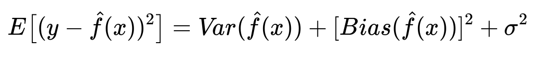
Where y is the true target, x is the input vector of features, \hat{f}(x) is the model’s prediction, Var(\hat{f}(x)) measures how much your model’s predictions fluctuate for different training sets drawn from the same distribution, [Bias(\hat{f}(x))]^2 represents how far off on average your model’s predictions are from the true target, and \sigma^2 is the irreducible noise inherent in the data that no model can capture.
In practical terms, you want to choose a model complexity that strikes a good balance. A very simple model (for instance, linear regression with few features or constraints) may have low variance but high bias, and likely underfits. A very complex model (for example, a large random forest with many trees or a deep neural network without enough regularization) can potentially overfit, exhibiting low bias but high variance.
When building models for loan approvals, you typically:
• Monitor overfitting through evaluation metrics on a separate validation set or via cross-validation. • Track underfitting by seeing if both training and validation accuracy remain low. • Employ techniques such as regularization (e.g., L1/L2 regularization), dropout (for neural networks), or pruning (for decision trees and random forests) to reduce high variance. • Increase model complexity or include more relevant features to reduce high bias if the model is clearly underfitting.
A key takeaway for this specific loan approval scenario is that different features vary in their usefulness. Features like credit score, income, and occupation probably have a strong influence on the model, while something like “favorite color” may add noise or lead the model to overfit if it picks up spurious correlations.
To find a suitable final model, you would carefully evaluate performance via a proper validation strategy, possibly cross-validation, and choose the model capacity and hyperparameters that balance the bias-variance tradeoff.
What if the data has many irrelevant features, like favorite color or height?
If your dataset has features that do not carry useful predictive information, the model may treat these irrelevant features as noise. This can inflate model variance because the model may overfit to random fluctuations in those features. You would typically apply feature selection or regularization methods to mitigate this risk. Techniques such as L1 regularization (lasso) force the model to shrink some coefficients toward zero, effectively ignoring irrelevant features.
How do you detect if you are overfitting or underfitting in practice?
In practice, you check performance metrics on both training and validation sets (or through cross-validation). If you see high training performance but significantly lower validation performance, this is a sign of overfitting. If performance is uniformly poor on both training and validation sets, it indicates underfitting. Monitoring learning curves is also helpful; if the training curve is high and the validation curve is significantly lower and not converging, overfitting is likely the culprit. If both training and validation curves converge to a similar low metric, underfitting could be the issue.
How can you handle a scenario where the data is limited?
When there is limited data, you risk high variance because the model might latch onto random noise in a small training set. Approaches to mitigate this include using cross-validation for more reliable performance estimates, applying strong regularization, or transferring knowledge from related tasks (transfer learning). Simpler models might be advantageous when data is very scarce to reduce the chance of overfitting.
Are there specific strategies to reduce model variance or bias?
To reduce variance, you can employ regularization, collect more data if possible, use simpler models, or use ensembling methods like bagging that can average out fluctuations across multiple models. To reduce bias, you can make the model more flexible, add more relevant features, or shift from simpler methods (like a single shallow decision tree) to more complex ones (like deeper trees or neural networks).
Why is the bias-variance tradeoff so critical for high-stakes applications like loan approvals?
Decisions like loan approvals have substantial real-world implications. Underfitting (high bias) might make the model overlook many worthy applicants. Overfitting (high variance) might approve high-risk borrowers. Striking the right balance ensures that genuinely qualified applicants are accepted, while the institution’s financial risk is properly managed. Additionally, interpretability can matter for regulatory compliance, so you must pay attention to the model’s complexity and ensure you can explain it if needed.
Below are additional follow-up questions
Could the bias and variance definitions change if the task is classification instead of regression?
For a classification setting like loan approval (approve vs. deny), the overall bias-variance intuition remains consistent, but the exact way these concepts manifest can differ slightly from regression. In classification, bias refers to how accurately the model separates classes on average across different training sets, while variance captures how much the decision boundary fluctuates with different samples. A high-bias classifier will consistently misclassify certain patterns, often using an oversimplified rule. A high-variance classifier may latch onto noise in the training data, shifting its decision boundary drastically with even small changes in the training set.
Pitfalls and Edge Cases • If the dataset is highly imbalanced (e.g., very few defaults), a model might appear to do well overall by predicting the majority class, thus showing low variance but potentially high bias. • In high-stakes tasks, misclassifying even a minority of applicants can have significant consequences, so a purely accuracy-focused bias-variance analysis might miss practical considerations like fairness and cost of misclassification.
How does data skew or class imbalance affect the bias-variance tradeoff?
When one class (e.g., “approved” loans) vastly outnumbers the other (e.g., “rejected” loans), many standard models tend to focus on the majority class, which can increase bias toward that class. Additionally, if the model overfits minority class signals, it might fluctuate too heavily in how it treats that minority, thereby increasing variance.
Pitfalls and Edge Cases • Oversampling or undersampling may help balance classes, but oversampling can make the model more prone to variance if duplicated minority samples dominate small regions of feature space. Undersampling can risk high bias if we discard too much data. • Advanced techniques like SMOTE (Synthetic Minority Over-sampling Technique) can help but require caution in how synthetic points are generated. Poor parameter choices can lead to synthetic points that do not reflect real-world applicants, adding noise and variance. • Class-weight adjustments in algorithms like logistic regression or tree-based methods can mitigate imbalance by penalizing misclassifications of the minority class more heavily, but tuning these penalties can be tricky and must be validated carefully.
If model interpretability is required, how does that interact with the bias-variance tradeoff?
Models like deep neural networks or large ensembles (e.g., random forests with hundreds of trees) may have lower bias but often at the expense of interpretability. Interpretable models (like simple decision trees or logistic regression) might have higher bias but be easier to explain. Deciding whether a more complex model is acceptable can depend on the regulatory and business environment.
Pitfalls and Edge Cases • Some explainability approaches (like LIME, SHAP) can approximate how complex models use features, but these approximations may have their own inaccuracies. • A complicated model with low bias and acceptable variance might still be rejected by regulators if it fails certain transparency criteria. • Simplifying a model just for explainability can introduce bias if we remove or approximate critical nonlinear interactions among features.
What if the underlying data distribution shifts over time (concept drift)?
Loan applicant behavior and financial climates can change due to macroeconomic factors, policy changes, or shifts in consumer habits. A model trained on historical data might gradually underfit as time passes, which is effectively an increase in bias—its assumptions no longer hold as well.
Pitfalls and Edge Cases • Sudden economic events, like a recession, can abruptly invalidate old patterns. Relying on outdated data can greatly increase bias because the model might have systematically wrong assumptions. • Gradual drifts are harder to detect; performance may degrade slowly, making it unclear whether to update the model or if the cause is random fluctuation. • Updating the model too frequently can introduce high variance, especially if each new dataset is small or includes noisy instances.
How do we handle cost-sensitive scenarios where the cost of false approvals is different from false rejections?
In many financial applications, incorrectly approving a bad loan (false positive) can be more costly than incorrectly denying a good applicant (false negative), or vice versa, depending on business objectives. Balancing this can impact the bias-variance tradeoff because you might allow the model to favor one type of error over another.
One way to capture this formally is via a custom cost function:

Where alpha and beta are positive weights indicating the relative cost of each type of misclassification. The model can be trained or tuned to minimize this custom cost instead of overall accuracy or error rate.
• \#False Negatives means the number of times the model denied a loan that should have been approved. • \#False Positives means the number of times the model approved a loan that should have been denied. • alpha and beta are the respective penalties or costs for these errors.
Pitfalls and Edge Cases • If alpha is too large, you might over-correct and end up approving more risky loans (increasing variance). • If beta is too large, you risk under-approving deserving applicants (increasing bias). • Estimating alpha and beta accurately can be difficult. If they are not grounded in real business or societal costs, the model’s predictions will be skewed in unhelpful ways.
How do ensemble methods (bagging, boosting) influence the bias-variance tradeoff?
Ensembling is often used to reduce variance by combining multiple diverse models (bagging) or iteratively refining weak learners (boosting). Bagging can lower variance significantly without a major increase in bias; boosting tends to reduce both bias and variance if each successive learner addresses errors from prior ones. However, in extreme forms (e.g., too many iterations in boosting), you can overfit.
Pitfalls and Edge Cases • Overly complex ensembles can become black boxes that regulators and stakeholders find non-transparent, complicating acceptance of the model. • Combining many weak learners that are individually high-bias might still lead to an ensemble that is too simplistic if those learners share the same bias. • If the training data is not large enough, boosting can chase noise, thereby increasing variance instead of reducing it.
What if domain experts disagree with the model’s predictions?
In high-stakes decisions, domain experts (loan officers, underwriters, etc.) may have nuanced insights about edge cases. If the model systematically disagrees with domain experts, it could reflect underfitting (high bias) or overfitting (high variance) for certain subpopulations. It may also reflect that experts use heuristics or partial data not captured in the training set.
Pitfalls and Edge Cases • Experts might have biases that the algorithm ironically corrects for, making direct “expert mismatch” a poor measure of error. • If experts rely on real-world knowledge not captured in the features, the model may miss an important dimension, leading to genuine bias or variance issues. • Continuous monitoring or a hybrid approach that factors in expert input alongside model outputs may be required to address high-risk or borderline applications.
How do you ensure that the model’s regularization or complexity controls do not eliminate critical features?
When applying methods like L1/L2 regularization or hyperparameter constraints (e.g., limiting the depth of trees), you reduce variance but risk increasing bias by discarding potentially important feature relationships. If the parameter controlling regularization strength is set too high, the model might ignore subtle but crucial signals.
Pitfalls and Edge Cases • Automatic feature selection or heavy regularization might eliminate critical demographic or financial indicators, hurting model performance. • In data-poor environments, regularization might collapse many feature coefficients, hiding signals from subgroups of applicants. • Cross-validation might show an overall performance improvement but still miss pockets of the population that become under-represented in the final model due to over-regularization.