
ML Interview Q Series: Hypothesis Testing: Understanding and Balancing Type I and Type II Error Trade-offs

Browse all the Probability Interview Questions here.
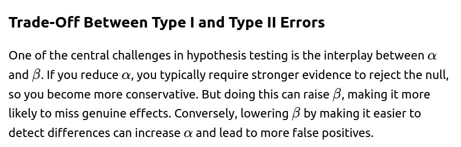
Explain the concepts of Type I and Type II errors in hypothesis testing and examine the trade-off that exists between them
Short Compact solution
Both types of errors arise in the setting of hypothesis testing. A Type I error happens when the null hypothesis is correct, yet we reject it. This is commonly referred to as a false positive. A Type II error occurs when the alternative hypothesis is actually true, but we fail to reject the null hypothesis. This corresponds to a false negative. In everyday terms, a Type I error means concluding there is a significant difference when none really exists, while a Type II error means missing a difference that truly is present.

Comprehensive Explanation
Overview of Hypothesis Testing
In statistical hypothesis testing, we typically have two main statements:


Understanding Type II Error
Type II error is the event where the null hypothesis is actually false (meaning the alternative is true), but the test fails to reject the null. The probability of committing this mistake is β. Missing a real effect that is present can be costly in many scenarios. Often, researchers prefer to design experiments with high statistical power, which is 1−β. A higher power implies a lower β, so there is a reduced probability of overlooking true differences.
Achieving low Type II error is directly connected to the design of the study. Factors that help reduce β include increasing the sample size, enhancing measurement precision, and making appropriate choices of statistical tests.
In practice, the right balance depends on the domain. For instance, in clinical trials for a life-threatening disease, failing to approve a truly effective treatment (Type II error) may be considered worse than approving an ineffective treatment (Type I error). In other scenarios, especially those involving high risk of false alarms leading to big costs, the focus might be on keeping Type I error low.
Role of Sample Size and Effect Size

Practical Implications
The cost of each type of error can be very different depending on context. For example:
In medical diagnostics, a Type I error might be falsely diagnosing a patient with a condition they do not have. A Type II error might be not diagnosing a patient who does have the condition. Each mistake can have different consequences: unnecessary treatments vs. missing life-saving therapies.
In fraud detection systems, a Type I error might block a legitimate transaction, while a Type II error might allow a fraudulent transaction to proceed.
In spam email filters, a Type I error is putting a legitimate email in the spam folder, while a Type II error is letting spam into the inbox.

Mathematical Summary


Potential Follow-Up Questions
How do confidence intervals relate to Type I error?

How do we reduce both Type I and Type II errors at the same time?
Are Type I errors always considered more serious than Type II errors?
How is the concept of p-value related to Type I error?


How does effect size influence Type II error?
If the true difference between groups or conditions (the effect size) is large, tests will more easily detect that difference, reducing β. When the effect size is very small, it can be harder to distinguish from random noise. Achieving low Type II error in such scenarios often requires large sample sizes or more refined measurement techniques.

Below are additional follow-up questions
How do Type I and Type II errors translate in settings where there is no explicit “truth” (e.g., certain unsupervised learning contexts)?
In some scenarios, such as clustering or anomaly detection in an unsupervised manner, there may be no clear-cut “true label” or accepted ground truth. This makes the notion of rejecting or failing to reject a null hypothesis less direct compared to a typical supervised hypothesis test.
Nevertheless, you can frame analogous concepts:
Type I Error: Declaring that some pattern (for instance, a cluster structure or anomaly) exists when, in a practical sense, it may not be meaningful or consistent in further analyses. For example, you might “split” the data into multiple clusters when they are actually random fluctuations in high-dimensional space.
Type II Error: Overlooking a pattern that does, in fact, exist, such as failing to identify an emerging cluster in your data.
A subtle pitfall is that in purely unsupervised methods, it is difficult to quantify these errors in a straightforward manner because you do not have a known distribution for the null hypothesis or a labeled set to confirm your findings. Often, one must either artificially introduce known signals (like simulated anomalies) to calibrate or rely on domain knowledge to gauge whether a discovered pattern is valid. For instance, a domain expert might give feedback about whether discovered clusters or anomalies make intuitive sense, partially addressing the possibility of Type I or Type II errors.
When switching between different test statistics or distributional assumptions, do Type I and Type II errors change?

Impact on Type II Error: Type II error depends on the power of the test. A test statistic that aligns better with the true data generating process or that more effectively captures the effect size will have higher power, leading to a lower chance of missing real differences. Conversely, a poorly matched test statistic or incorrect assumptions (e.g., using a t-test with heavily skewed data and small sample size) can inflate β and increase the Type II error rate.

In Bayesian frameworks, how do priors influence the balance between Type I and Type II errors?
Bayesian hypothesis testing does not typically classify outcomes in terms of Type I or Type II errors in the same manner as frequentist approaches. Instead, one updates belief about parameters or models by combining priors with the likelihood of the observed data. However, if we mirror the idea of “rejecting or accepting a hypothesis” in a Bayesian sense—perhaps by deciding if a posterior probability surpasses a threshold—priors can significantly shift the effective “false positive” and “false negative” rates:
Influence on ‘False Positive’: A strong prior that heavily discounts the possibility of an effect can make it harder for the posterior to rise above the threshold needed to accept that effect. This corresponds to reducing the risk of incorrectly concluding there is an effect (a Type I error analog), but it might also increase the risk of missing a real effect (a Type II analog).
Influence on ‘False Negative’: If the prior strongly favors the presence of an effect, the posterior might remain supportive of the effect even with moderate evidence, thereby reducing the chance of failing to detect a true effect.
An additional real-world edge case is selecting an inappropriate or dogmatic prior. For instance, if a prior is too narrow (or unrepresentative of genuine possibilities), it can cause the Bayesian analysis to produce systematically skewed posterior inferences, effectively distorting both ‘false positive’ and ‘false negative’ outcomes in ways that are hidden from a purely frequentist perspective.
How can dynamic or time-varying costs of errors affect Type I and Type II error control?
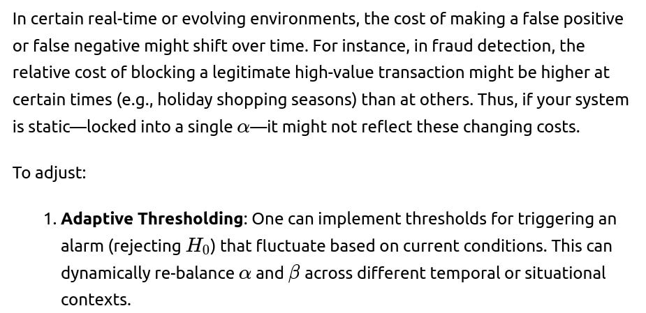
2. Contextual Priorities: Using domain-based heuristics, the system can weigh false positives and false negatives differently at different times. This approach is reminiscent of cost-sensitive learning in machine learning, where misclassification of certain classes has higher or lower cost.


A subtlety arises when the method for adjusting thresholds introduces multiple sequential “tests,” each with its own chance to produce an error. Over many dynamic adjustments, controlling the global Type I or Type II error rate consistently can be tricky. Additionally, abrupt changes or non-stationarity in the data distribution might lead to unanticipated spikes in either false positives or negatives if the system is not robustly calibrated.
How do we manage Type II errors in practice when the true effect size is uncertain?
When planning a study or experiment, researchers often try to estimate the sample size required by hypothesizing a certain expected effect size. But if the actual effect size deviates from the initial assumptions—e.g., it is smaller than anticipated—then the test might become underpowered, leading to a high risk of Type II errors.
Practically:
Pilot Studies: Running smaller, preliminary studies allows a more realistic estimate of the effect size. However, pilot data might still suffer from sampling error or limited generalizability.
Sequential or Adaptive Designs: Methods such as group sequential designs allow researchers to periodically check interim results and possibly adjust the sample size. This can help rectify an initial underestimation of effect size.
Bayesian Updating: As data accumulates, you can update your beliefs about the effect size. If it appears smaller, you might increase the sample size or refine your measurement protocols to avoid missing true effects.
Pitfalls include misinterpreting pilot results (for example, concluding a large effect size if the pilot sample was unrepresentative) and adopting an overly flexible adaptive design that might inflate Type I error if not carefully controlled.
How do Type I and Type II errors manifest in multi-metric A/B tests?
In A/B testing, you may measure multiple outcomes—such as click-through rates, session duration, and conversion rates—on the same experiment variants. Each metric tested separately has its own probability of Type I and Type II errors. But collectively:
Inflated Type I Error: Testing many metrics in parallel increases the chance of finding a significant difference on at least one metric purely by chance. Without correction, this can lead to a spurious conclusion (false positive) that a new variant outperforms the control.
Complex Type II Error Patterns: Even if there is a true improvement in one or more metrics, applying multiple-comparison corrections (e.g., Bonferroni, Holm’s method) can become conservative and might overlook some real improvements. This risk elevates the chance of missing subtle but genuine gains across multiple metrics, effectively increasing Type II errors.
A nuanced challenge is that these metrics might be correlated; thus, standard multiple-comparison corrections might be either overly or insufficiently strict. Approaches like MANOVA or hierarchical models can account for these correlations, but they introduce more complexity to the analysis.
Can Type I and Type II errors change over time in real-time detection or streaming contexts?
Yes. In many streaming contexts—like real-time anomaly detection or intrusion detection—data arrives continuously, and you often apply repeated checks. Each check can produce its own Type I or Type II error. Over thousands or millions of time points:

Adaptive Type II Errors: As conditions shift (concept drift in machine learning), a static detection rule might gradually lose power to detect genuine anomalies or attacks.
Online learning or sequential hypothesis testing methods (e.g., the CUSUM test for drift detection) can help maintain control over error rates by adjusting thresholds based on recent observations. However, these methods typically assume certain stationarity or rely on heuristics to adapt to changing distributions. A subtle pitfall is that abrupt and large distribution shifts can cause dramatic spikes in false positives or negatives until the system fully recalibrates.
In predictive modeling, how do Type I and Type II errors link to metrics like precision, recall, and F1 score?
In a typical binary classification model, a Type I error corresponds to predicting “Positive” when the ground-truth is actually “Negative,” while a Type II error corresponds to predicting “Negative” when it is actually “Positive.” These map directly onto the confusion matrix:
Precision: Reflects, out of all predicted positives, how many are truly positive. High precision implies a low rate of Type I errors with respect to the predicted positives.
Recall: Indicates, out of all actual positives, how many were correctly identified. Low recall means high Type II errors.
F1 Score: A balanced measure capturing both precision and recall, thereby reflecting a trade-off between Type I and Type II errors.
A hidden complication arises when data is highly imbalanced. In scenarios where the positive class is very rare (e.g., fraud detection), a model can have seemingly excellent precision yet still miss most actual positives. Similarly, if you optimize heavily for recall, you can drastically raise the false positive rate. Aligning the classification threshold with domain-specific cost or risk helps manage these trade-offs in a practical manner.
How does sequential hypothesis testing address repeated analyses of the same data, and why is it tricky for error rates?
Sequential testing allows you to check accumulating data at multiple interim points (often to decide whether to terminate or continue a study early). While this practice is efficient, it complicates Type I error control because each additional look at the data increases the chance of a false positive:
Inflated Type II Error: Using overly conservative boundaries might increase the risk of missing a real effect (Type II error). Conversely, some designs can enhance power, but they must be carefully designed and documented upfront to avoid “p-hacking” or data snooping.
The main pitfall is unplanned interim analyses without proper error-rate adjustments. Doing so can lead to researchers stopping the trial prematurely the first time a significant result appears, effectively inflating the chance of a Type I error well above the nominal level.
How do multi-dimensional data or multiple data sources complicate Type I and Type II errors?
In real-world scenarios, you may combine multiple streams of data—text, images, numerical logs—from different systems or sensors. Each source might have its own distribution and correlation structure with other sources:
Risk of High-Dimensional Noise: As the dimensionality grows, small-sample statistical properties may degrade. Tests might detect spurious differences (Type I errors) if not carefully regularized or controlled.
Correlation Structure: If the data sources are correlated, certain signals may be counted more than once, inflating false positives. Conversely, if you incorrectly assume independence and ignore overlapping information among data sources, you might fail to detect true signals, increasing Type II errors.
Feature Selection or Dimensionality Reduction: Techniques like PCA or feature selection can help reduce noise but might inadvertently discard relevant signals, thereby increasing Type II errors if not done carefully. If you optimize feature selection to minimize Type I error, you could underfit or ignore subtle patterns.
A typical subtlety occurs in sensor fusion: combining multiple sensors can enhance detection power (reducing Type II error), yet it may also introduce complex correlations or biases that inflate Type I error unless carefully handled.