ML Interview Q Series: Hypothesis Testing Explained: Understanding P-values for Statistical Significance

Browse all the Probability Interview Questions here.

How would you explain the idea of hypothesis testing and the role of p-values in plain language?

Short Compact solution

The practice of determining whether the observed data supports specific assumptions is called hypothesis testing. It usually involves measuring some feature of interest from at least two groups: a control group that does not receive a particular treatment and another group (or more) that does receive it. In many scenarios, this could be something like comparing two sets of people based on their average height, conversion rates of different user flows in a product, or comparing any other measurable quantity.

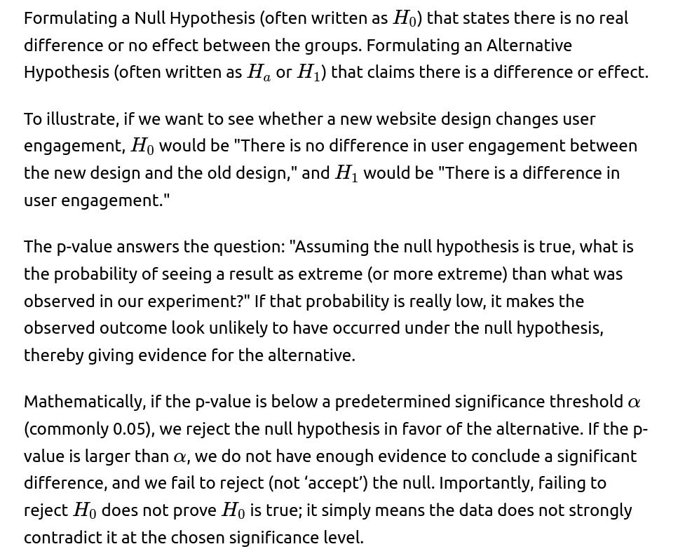
When conducting the test, two opposing claims are formed. The null hypothesis states there is no meaningful difference or effect between the groups, while the alternative hypothesis assumes that a true difference or effect exists due to the treatment or condition applied.

A p-value represents how likely it would be to see the observed results (or something more extreme) if the null hypothesis were correct. A small p-value indicates that such observed data would be quite improbable under the null hypothesis. If the p-value is below a chosen significance level (often 0.05), it suggests rejecting the null hypothesis in favor of the alternative. Otherwise, we do not have enough evidence to claim any significant difference or effect.

Comprehensive Explanation

Hypothesis testing is a cornerstone of statistical inference. In simple terms, a researcher proposes a question: "Does a certain factor (like a new drug, a website design change, or a marketing campaign) cause a difference in some measurable outcome (like recovery rate, click-through rates, or sales)?" This question is investigated by collecting data from groups that either do or do not experience the factor. The main steps include:

Potential Follow-up Question: Could you give an example of how to compute and interpret p-values using Python?

An example in Python, using the SciPy library, could look like this:

import numpy as np
from scipy import stats

# Sample data: two independent groups
group_a = np.array([5.1, 4.9, 5.0, 5.2, 5.3, 5.1, 4.8])
group_b = np.array([5.5, 5.7, 5.6, 5.4, 5.6, 5.5, 5.8])

# Perform an independent two-sample t-test
t_statistic, p_value = stats.ttest_ind(group_a, group_b)

print("T-statistic:", t_statistic)
print("p-value:", p_value)

alpha = 0.05
if p_value < alpha:
    print("Reject the null hypothesis. There is a significant difference.")
else:
    print("Fail to reject the null hypothesis. No significant difference found.")

Potential Follow-up Question: How do you decide which test to use?

Choosing the appropriate hypothesis test depends on various factors:

Whether data in each group are independent or paired (e.g., measuring the same subjects before and after a treatment). The data distribution. For large sample sizes, the Central Limit Theorem helps many tests to be relatively robust to normality assumptions. For smaller sample sizes, normality assumptions matter more. Whether we are dealing with categorical or numerical data. For categorical data, tests like the chi-square test may be used, while for numerical data with two groups, a t-test is common if normal assumptions hold, or a non-parametric test like the Mann-Whitney U test if they do not.

Potential Follow-up Question: Why do we sometimes use a significance level of 0.01 instead of 0.05?

Potential Follow-up Question: Are p-values the final word on whether a result is important?

No. Statistical significance is not synonymous with practical importance. A very large sample size can yield a statistically significant difference for an effect that is too small to matter in a real-world setting. Researchers often supplement p-values with confidence intervals and effect size measurements to gauge the real-world impact.

Potential Follow-up Question: What are one-tailed and two-tailed tests?

A one-tailed test checks for an effect in a specific direction (e.g., "the new design is better than the old one"). A two-tailed test checks for an effect in either direction (e.g., "the new design is simply different, whether better or worse"). Choosing between one-tailed and two-tailed tests depends on the research question. Two-tailed tests are more conservative, because splitting the significance level across two directions makes it harder to reach significance unless you see a strong effect in one specific direction.

Potential Follow-up Question: How does multiple hypothesis testing affect p-values?

Below are additional follow-up questions

What if the distributional assumptions (like normality) are not valid for the chosen test?

When a hypothesis test assumes normality or other specific distributional properties, and the actual data deviate from those assumptions, the resulting p-values can be misleading. For example, a t-test assumes that the data in each group follow approximately normal distributions and have reasonably similar variances. If your data have heavy tails or show strong skewness, a t-test might overestimate or underestimate the p-value, leading to incorrect conclusions.

A practical way to address this problem is to use non-parametric tests (like the Mann-Whitney U test for two independent groups or the Wilcoxon signed-rank test for paired samples) which do not rely so strictly on normality. If sample sizes are large enough, the Central Limit Theorem often helps justify normal-based tests, but it is still good to perform exploratory data analysis—like plotting histograms, Q-Q plots, or performing formal normality tests—to confirm assumptions. Another pitfall arises with small sample sizes; the normality assumption is much more critical when you have fewer observations, since the Central Limit Theorem is less reliable.

Additionally, in real-world tasks such as measuring time-to-event (survival analysis) or count data (Poisson assumptions), specialized statistical methods can more robustly handle those distributions. Ensuring the correct model specification is crucial to obtaining a valid p-value.

How do Bayesian approaches differ from frequentist p-values?

Frequentist hypothesis testing with p-values tries to answer the question: “If the null hypothesis is true, how unusual are the observed (or more extreme) data?” By contrast, Bayesian approaches compute the posterior probability of hypotheses given the data, usually expressed as P(hypothesis∣data).

In a Bayesian test, one typically specifies a prior belief about the parameters or model. The data update that prior to form the posterior distribution. Then you might ask questions like: “What is the probability that the parameter is greater than some threshold?” In other words, while frequentist p-values are about data extremity under an assumption, Bayesian methods are about the probability of hypotheses themselves.

A potential pitfall is that defining priors can be somewhat subjective. However, when priors are carefully chosen (or if you use non-informative or weakly-informative priors), Bayesian analysis offers a direct interpretation of the probability of your hypothesis. This distinction is critical in real-world tasks that require explicit probability statements about parameters, such as medical diagnostics or risk analysis.

How do we account for sequential testing or stopping rules in A/B experiments?

In many real-world A/B tests, analysts frequently peek at the results during the test period and may stop the experiment once they see a “significant” difference. Standard p-values assume a fixed sample size determined before the test begins. When you deviate from that plan (e.g., checking daily and stopping early), you inflate the probability of a false positive.

To correct for this, one strategy is to use group sequential methods or methods like alpha spending functions that adjust your significance threshold each time you peek at the data. Another approach is Bayesian A/B testing, which can incorporate flexible stopping rules. A widely used practical solution is to define a minimum test duration and sample size before analyzing the results and to resist the temptation of interpreting interim p-values as final evidence.

How do confounding variables affect hypothesis testing and p-values?

A confounding variable is a factor not accounted for in your experimental design that might systematically affect the results. If you fail to control or randomize these confounding factors, your p-values might reflect the effect of these confounders rather than the effect you intended to measure. For instance, if you test a new marketing strategy in one geographic region only, but that region has distinct customer behaviors, observed differences might be driven by geography rather than the strategy.

Randomization is a key tool to mitigate confounding variables, ensuring that both known and unknown confounders are distributed roughly evenly across experimental groups. When randomization isn’t possible, methods like stratification, matching, or regression adjustments can help isolate the effect of interest. Still, if confounding variables are not properly addressed, your p-values may be misleading, incorrectly suggesting significance (or lack thereof).

How do we measure practical significance alongside statistical significance?

Statistical significance tells you if an observed effect is unlikely to be due to chance, while practical significance asks whether that effect truly matters in the real world. To assess practical significance, researchers use measures like effect size (Cohen’s d for differences in means, or odds ratios for binary outcomes) and confidence intervals. For example, if you find a p-value of 0.001 indicating a very small p-value, but the difference in means is 0.01 on a scale of 0–100, that difference may be statistically significant but practically irrelevant.

One subtle issue arises if you have an extremely large sample size: even trivial effects can become “significant.” Conversely, if you have a very small sample, important effects might go undetected if they do not reach significance due to limited power. Reporting confidence intervals along with effect sizes helps avoid these pitfalls by revealing the magnitude and precision of the effect, rather than focusing solely on p-values.

What is the difference between one-sample, two-sample, and paired tests?

A one-sample test compares observed data against a known or hypothesized population parameter. For example, you might test whether the average weight in a sample of products is equal to a target specification.

A two-sample test compares two independent groups. For instance, comparing average blood pressure between a control group and a treatment group.

A paired test is used when the same subjects or units are measured twice under different conditions, making the measurements dependent. An example would be measuring a patient’s cholesterol level before and after starting a new medication. This repeated-measures setup increases statistical power but also changes the structure of your null hypothesis (differences within pairs rather than differences across independent groups).

A subtle pitfall is mixing up independent-sample t-tests with paired t-tests when the data are actually paired. This can lead to incorrect p-values. Another scenario arises when the data are correlated in some other way and an appropriate paired or repeated-measures design is not properly accounted for.

Why is it crucial to distinguish correlation from causation in hypothesis testing?

Hypothesis tests can show an association (i.e., correlation) but do not inherently establish causation unless the study is designed for it (e.g., randomized controlled trials). Even if a p-value is extremely small, it only indicates a statistical relationship under the null hypothesis; it doesn’t prove that one variable causes the other. Other unobserved confounding factors may be driving the association.

Failing to distinguish correlation from causation can lead to unwarranted conclusions, such as attributing a change in user behavior to a marketing campaign when, in reality, there was a seasonal effect or some other coincidental external factor. Control groups, randomization, and careful design are key to inferring causality. Even then, statisticians often use language like “provides evidence for a causal effect” rather than “proves” it, because unmeasured confounders can still exist.

How do we handle the scenario of multiple metrics within a single A/B test?

In many A/B tests, multiple performance metrics are tracked, such as click-through rates, time on site, conversion rates, etc. Testing each metric independently can lead to multiple comparisons issues, inflating the likelihood of false positives. For instance, if you track 10 metrics at a significance level of 0.05, even if all differences are due to chance, there is a substantial probability that at least one will appear significant.

To mitigate this, adjustments like the Bonferroni correction or a False Discovery Rate (FDR) method can be applied, lowering the threshold for significance across multiple metrics. Another approach is to define a primary metric beforehand (the one that drives your main business goal) and consider secondary metrics for exploratory analysis. By pre-registering your main outcome measure, you reduce the chance of selectively reporting a “significant” metric that emerges by chance.

Does repeatedly tuning and retesting a model or hypothesis lead to overfitting in statistical testing?

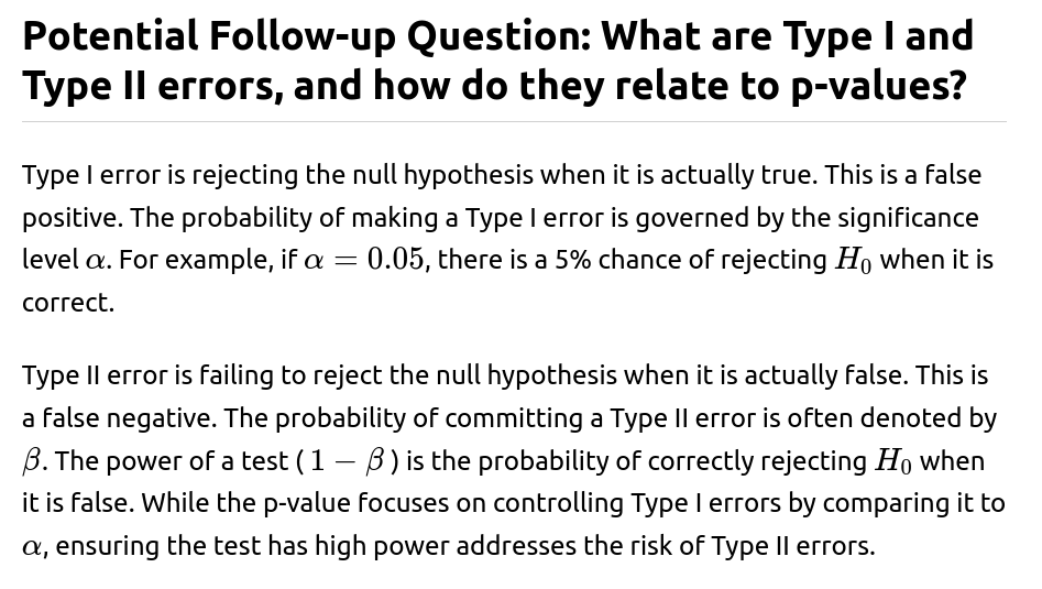
Yes. If you test a hypothesis, observe the results, tweak your model or data collection, and then retest the same hypothesis on the same data, you are effectively “overfitting” the data from a statistical standpoint. Each iteration can inflate the Type I error rate, making it more likely to see a significant result by chance alone.

One solution is to conduct a fresh test on new data whenever you modify your approach. Alternatively, you can use formal procedures such as cross-validation to separate model-building from final evaluation. This separation ensures that your final p-value or statistical test is unbiased by the iterative tuning process. In real-world machine learning, a train/validation/test split or nested cross-validation is often used to prevent inflating performance estimates due to repeated hyperparameter tuning on the same dataset.

What is p-hacking, and how can we avoid it?

P-hacking refers to a range of practices that artificially produce or inflate statistical significance. Examples include running many different tests or data transformations and selectively reporting the ones that yield a small p-value, stopping data collection as soon as a significant result appears, or excluding outliers only after seeing how they affect significance.

These practices can mislead you into believing you’ve found a meaningful result when you have not. To avoid p-hacking, researchers can pre-register their hypotheses, data collection methods, and analysis plans. They can also apply corrections for multiple comparisons or use more robust approaches like Bayesian inference. Documentation and transparency about all analyses performed help reduce the temptation or ability to selectively report only significant findings.