ML Interview Q Series: Hypothesis Testing for Coin Bias Using Normal Approximation

Browse all the Probability Interview Questions here.
A coin was tossed 1000 times, and 550 of those outcomes were heads. Should we conclude that the coin is biased, and why or why not?
Short Compact solution
Because the number of flips is large, the distribution of heads can be approximated by a normal distribution, with mean 500 and standard deviation of about 16 (assuming a fair coin with probability p=0.5). Observing 550 heads implies a difference of 50 from the expected mean, which is about 3 standard deviations away (z≈3.16). In a normal approximation, such an outcome would be extremely unlikely (less than 0.1% chance) if the coin were truly fair. Hence, the coin is likely biased.
Comprehensive Explanation
Intuition and Underlying Concepts
When flipping a coin repeatedly, each individual flip can be seen as a Bernoulli random variable taking the value 1 if the flip is heads and 0 if it is tails. The total number of heads in n flips is then modeled by a binomial distribution if the flips are independent and the coin has the same probability p of landing heads on each flip.
If the coin is fair (p=0.5), we would expect on average half of the flips to be heads. Over n=1000 flips, the expected value (mean) of the number of heads is:


Using the Normal Approximation
For sufficiently large n, the binomial distribution can be approximated by a normal distribution with the same mean and variance (Central Limit Theorem). Therefore, we approximate the total number of heads by a normal distribution with mean 500 and standard deviation 16.
Observing 550 heads is 50 more than the expected mean of 500. We compute the z-score:

A z-score of around 3.125 to 3.16 corresponds to a very small two-tailed p-value (significantly less than 1%). This indicates that if the coin were truly fair, the likelihood of seeing such an extreme result is extremely low.
Conclusion from This Approach
Because the result (550 heads out of 1000) is so many standard deviations away from the mean predicted by a fair coin model, we have a strong indication that the coin might indeed be biased. Of course, in a real statistical setting, one would compute the exact p-value or set a confidence interval and then decide whether to reject the hypothesis of fairness at a chosen significance level. But from a quick rule-of-thumb normal approximation, a z-score over 3 is already highly suggestive that p=0.5 is inconsistent with the data.
Possible Follow-Up Questions
How is hypothesis testing formally applied here?
A formal approach uses a hypothesis test:
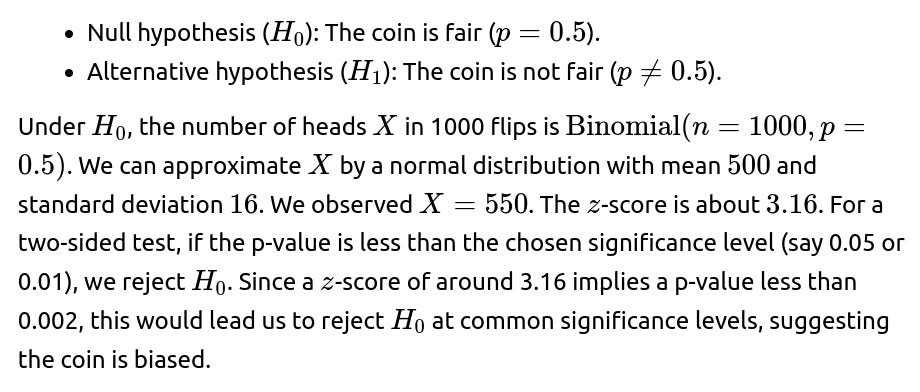
What if we questioned the independence of flips?
If the flips are not truly independent, the binomial model no longer strictly applies. For example, if the coin has a memory effect or if there is a mechanical process causing correlation between flips, the distribution of heads could deviate from the binomial assumption. In practical terms, you would need to investigate the flipping mechanism, or re-sample under more controlled conditions. In an interview, it’s good to note that the entire analysis hinges on independence and identical distribution of each flip.
Why do we assume the normal approximation is valid?
For large n, the binomial distribution tends to be well-approximated by a normal distribution due to the Central Limit Theorem. The rule of thumb is typically that both np and n(1−p) should be at least 10 (some texts say 5). Here, np=500 and n(1−p)=500 when p=0.5, so the normal approximation is quite accurate.
Could we use alternative methods without the normal approximation?
Yes. One could use an exact binomial test:
import math
from math import comb

def exact_binomial_test(n, k, p=0.5):
    # Probability of exactly k heads out of n using the binomial formula
    return comb(n,k)*(p**k)*((1-p)**(n-k))

# We could sum probabilities for all k >= 550 and k <= 450 (two-sided)
# to get the exact p-value.
# This can be computationally feasible for n=1000, but might require big integer handling or
# a library function in practice (e.g., scipy.stats).
In real practice, we might use a library like scipy.stats.binom_test in Python to get the exact p-value. The normal approximation is sufficient for quick mental or whiteboard calculations, but if you want the precise result, exact methods are available.
How to interpret practical significance vs. statistical significance?
In an interview, it’s worth emphasizing that a highly statistically significant result (like a z-score of over 3) strongly suggests that the coin is biased away from 0.5. However, the degree of bias might be small. For instance, the empirical estimate of p is 550/1000=0.55. That’s a 10% deviation from 0.5 in relative terms, which is definitely large enough to be noticeable in gambling contexts or in applications where fair coins matter. But sometimes, even a smaller deviation could be practically important depending on the real-world situation.
Does the normal approximation break down if the coin is extremely biased?
Yes, if the true p is very close to 0 or 1, then the distribution of heads becomes skewed, and the normal approximation might be less accurate for moderate n. But with p=0.5 or near that, and n=1000, the approximation remains strong.
Would we need to check for a one-sided or two-sided deviation?
Often, interviewers may ask you to clarify if you suspect the coin is biased towards heads or tails specifically. A one-sided test would check if the coin lands heads more than 50% of the time, whereas a two-sided test is for “any” bias. Since we do see an excess of heads, a one-sided test would make sense if we specifically hypothesized “the coin is biased towards heads.” This can slightly affect the calculation of the final p-value (roughly half of the two-sided p-value if the data go in the predicted direction). Clarifying these details in an interview is essential.
Could random variation sometimes produce results like 550 out of 1000 for a fair coin?
Yes, random variation can theoretically produce nearly any outcome, but it becomes highly improbable as you move many standard deviations from the expected mean. This is exactly the principle behind statistical inference: if data seem too improbable under the null hypothesis, we conclude that the assumption is likely wrong.
Real-world testing or practical considerations
Physical bias: Real coins can be physically biased. For instance, some trick coins or coins that spin differently on one side.
Experimental design: Are we flipping the coin by hand, using a mechanical flipper, or letting it spin on the table? The method can influence the fairness.
Systematic error: Could the method of counting heads be biased or misrecorded?
In an interview, mentioning these real-life factors shows that you understand practical issues beyond the pure math.
Below are additional follow-up questions
How might the coin’s bias change over time, and how would that affect our conclusion?
In some real-world situations, the probability of landing heads (p) might not remain constant across all flips. For example, if the coin is gradually warping, wearing out, or if environmental conditions (like the force with which the coin is flipped) are changing over time, then p could shift mid-experiment.
Impact on Independence and Identical Distribution The binomial model assumes each flip is independent with the same probability of heads. If p changes over time, we no longer have identical distributions across flips. As a result, the binomial (or normal approximation) analysis might not be strictly valid.
Detecting Gradual Shifts One way to detect changes is to split the 1000 flips into segments (e.g., first 250 flips, next 250 flips, etc.) and compare the observed heads rates in each segment. A changing bias might reveal itself as a trend in the proportion of heads across segments.
Statistical Models for Non-Stationary Processes If we suspect p varies with time, we could use methods designed for non-stationary data, such as a time-varying parameter model or a Bayesian approach with a dynamic prior. These can incorporate the possibility that p slowly drifts from flip to flip.
Pitfalls

In an interview, acknowledging that real processes can evolve over time demonstrates an understanding that real-world data often violate simple assumptions, requiring more sophisticated testing.
Why might a Bayesian approach be beneficial, and how would we apply it?
A Bayesian approach updates our belief about the coin’s probability of heads, p, as we observe more flips. Instead of just deciding “biased” or “not biased,” we get a posterior distribution for p.
Bayesian Framework
We begin with a prior distribution on p (e.g., a Beta(1,1) prior if we are initially completely uncertain and want a uniform distribution from 0 to 1).
As we observe heads (H) and tails (T), we update the distribution to obtain the posterior. For a Beta prior and Bernoulli likelihood, the posterior is also Beta, with parameters that reflect the observed heads and tails.
Benefits
We obtain a full distribution for p instead of just a point estimate or a binary decision. This distribution tells us how probable it is that p lies in any interval (e.g., above 0.5).
We can incorporate prior beliefs (like if we suspect the coin to be near-fair, or if we suspect it to be heavily biased) in a mathematically consistent way.
Drawbacks
The interpretation of priors requires careful thought; a poor choice of prior can overly influence the conclusion.
Bayesian computations can be more intensive if one does not use conjugate priors or if n is large and the problem is more complex (though for a coin flip scenario, the Beta-Bernoulli conjugacy is very convenient).
Edge Cases
Extremely small or large prior parameters might artificially skew the posterior.
If we have contradictory data (e.g., most flips show heads but the prior strongly favors p=0.5), the posterior eventually moves away from the prior if enough flips are conducted, but the number of flips required depends on the strength of the prior.
Being able to explain a Bayesian approach, especially in an interview, shows strong grasp of both frequentist and Bayesian paradigms, and how they can be applied to a simple coin flip scenario.
How many flips would we need if we want to detect a smaller bias with the same statistical confidence?
Often, we are interested in the power of a test or how many trials are necessary to detect a specified deviation from 0.5.


Power Analysis Suppose you want to detect that p=0.51 (a 1% deviation) vs p=0.5 with 95% confidence and 80% power. You’d find that the required n is quite a bit larger than 1000 because distinguishing 0.51 from 0.50 is harder than distinguishing 0.55 from 0.50.
Practical Implementation
Testing for smaller biases might require thousands or even tens of thousands of flips. That might be time- or resource-consuming.
In an interview context, you can mention how a formal power analysis can guide whether it’s worthwhile or practical to gather more data.
Pitfalls
If the coin or environment changes over the course of many flips, you might not be measuring the same p.
Overlooking the cost and feasibility of performing so many flips.
Discussing sample size and power highlights the practical constraints of real testing scenarios and that significance is not just about the observed difference but also about how much data we’ve collected.
How might constructing a confidence interval help us interpret the result differently?
Instead of a hypothesis test (where we say “accept” or “reject” a null hypothesis), we can build a confidence interval for the true proportion of heads.
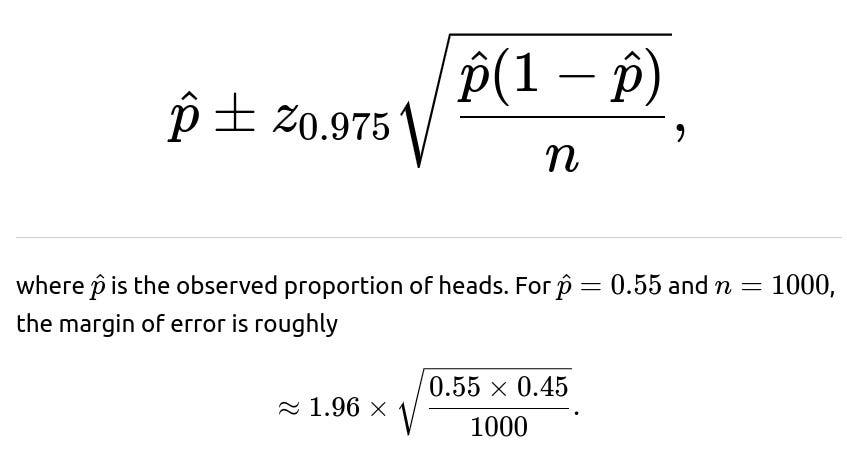
Confidence Interval for p A common approximate approach for a 95% confidence interval for p is:

Numerically, that’s about 0.03, meaning the 95% confidence interval is approximately [0.52, 0.58].
Interpretation This interval suggests that the true p could reasonably be anywhere from about 0.52 to 0.58. Since 0.5 is not in that interval, it supports the conclusion that the coin is likely biased.
Potential Pitfalls
Misinterpretation: a 95% confidence interval does not mean there is a 95% probability that p is in that interval (that’s a Bayesian statement). It means that if we repeated this procedure many times, 95% of such constructed intervals would contain the true parameter in the long run.
Small-sample corrections: for smaller n, alternative intervals or exact methods (e.g., Clopper-Pearson) may be more appropriate.
Using confidence intervals is an alternative to direct hypothesis testing and can offer a more nuanced view of the plausible range for p. That is an important distinction to understand thoroughly for real statistical conclusions.
How does the presence of potential measurement or recording errors impact the analysis?
In some real-world studies, especially large-scale experiments or data collection settings, there might be errors in measuring or recording the outcome (e.g., mislabeling a head as a tail).
Types of Error
Random misclassification: Each flip outcome has some chance of being recorded incorrectly, but this chance does not depend on whether it’s heads or tails.
Systematic bias: More heads might be systematically recorded as tails or vice versa, depending on some observer bias.
Effect on Results
Random misclassification tends to dilute the observed difference from 0.5, making it harder to detect a true bias.
Systematic bias can either artificially inflate or deflate the observed difference from 0.5, potentially leading to false conclusions about bias.
Possible Remedies
Double-check flipping and recording procedures, or use automated methods (e.g., computer vision counters).
Model the error rate. If we suspect a certain small probability of misclassification, we can incorporate that into a corrected analysis (though that becomes more complex statistically).
Pitfalls
Failing to account for measurement error can lead to inaccurate p-value calculations.
Over-correcting for suspected biases if we lack data to estimate the magnitude of such errors.
An interviewer might test your awareness that real data can be messy and that perfect measurement is rarely guaranteed, especially if you are dealing with hardware or observational data.
Could the flips themselves influence future flips (e.g., momentum effects), and how to handle such dependencies?
Sometimes, in physical processes, the exact spin or flip might carry momentum to the next flip. If the experiment isn’t reset each time, the flips could be correlated.
Violation of Independence A fundamental assumption in binomial sampling is independence of flips. If flips are correlated, the variance might be different from np(1−p). We might see streaks of heads (or tails) more frequently than expected under independence.
Statistical Tests for Autocorrelation
We can examine the sequence of flips and apply tests like the runs test or compute autocorrelation coefficients at various lags.
If a significant autocorrelation is present, the standard binomial model is invalid.
Possible Solutions
Redesign the flipping mechanism to ensure independence (e.g., a fair coin-toss machine that carefully restarts from the same initial position each flip).
Use time-series or Markov models if correlation can’t be removed. These models incorporate the dependence in the flipping process.
Edge Cases
High correlation might render normal or binomial approximations inaccurate. The distribution of heads is no longer well described by the binomial formula.
Low correlation (small but nonzero) might not drastically alter conclusions unless n is huge.
Bringing up correlation among flips shows advanced statistical thinking and that you realize real-world processes do not always match ideal assumptions.
What if another coin was tested concurrently, also showing a deviation in heads. How do we handle multiple comparisons?
Often in practical experimentation, we may be testing multiple coins simultaneously or performing several statistical tests in parallel.
Multiple Hypothesis Testing Problem Each test has some chance of a false positive. When we run many tests (say, 10 or 100 coins), the chance that at least one test incorrectly indicates a bias grows. This leads to issues like the “multiple testing” or “false discovery rate” problem.
Statistical Corrections

Benjamini-Hochberg: A more nuanced approach that controls the false discovery rate rather than the family-wise error rate.
Pitfalls
Being unaware of multiple comparisons can lead to concluding that many coins are “biased” purely by chance.
Over-correcting can make detection of genuine biases harder.
Interviewers often check if candidates are aware of multiple hypothesis testing pitfalls, especially in big data or high-throughput scenarios.
How might prior knowledge of the coin’s manufacturing process influence our statistical analysis?
Sometimes, we know something about how the coin is made: for example, a minted coin from a reputable source is generally quite fair, whereas a coin from a novelty shop might be more suspicious.
Incorporating Prior Knowledge If we trust standard currency coins to be near-fair, we might expect p to be in a narrow range around 0.5. In a Bayesian framework, we could choose a prior centered around 0.5 with a moderate variance, reflecting our confidence. In a frequentist setup, we might shift our significance thresholds because we strongly suspect fairness.
Confirmation Bias Risk If we are too convinced that the coin is fair, we might underweight evidence that it’s actually biased. Conversely, if we suspect a trick coin, we might overemphasize small deviations from 0.5.
Pitfalls
Letting subjective biases override data.
Not gathering enough data because we rely too heavily on assumptions.
This question can reveal whether the candidate is aware of practical, domain-specific knowledge that can refine or skew statistical testing.
If we suspect a double-headed coin, how would we test that specifically?
Double-headed coins are sometimes used in magic tricks or gambling cheats, meaning p could be 1.0 (always heads).

Edge Cases
If p is extremely close to 1 but not exactly 1, then you might see a tail eventually, but perhaps after many flips.
Testing a double-tailed coin is analogous (looking for heads) but typically less common.
In practical or interview scenarios, such a trick coin question might test whether you can quickly deduce that one counterexample (a single tail) suffices to reject p=1.
If we need to detect a directional bias (i.e., the coin might be heavier on one side), how do we investigate that aspect physically?
A follow-up might challenge you to tie statistical inferences to physical or mechanical causes.
Physical Inspection
Weigh the coin or measure thickness. If the coin is heavier on the heads side, it could systematically affect flipping.
Check the center of mass if the coin’s shape is not perfectly symmetrical.
Statistical vs. Physical Explanation Even if data shows p=0.55, a good statistician or ML practitioner often wants a physical explanation. The mechanical cause can confirm if the result is a consistent phenomenon rather than a random anomaly.
Pitfalls
If the coin is slightly heavier on one side, real flipping might amplify or reduce that effect depending on flipping technique.
Overlooking that a biased result could be from a non-random flipping methodology (e.g., if the same person flips the coin in a consistent manner favoring one side).
Bringing physical reasons into the interview discussion shows awareness that not everything is purely random: real processes involve physics that can cause systematic bias.
What if we tested a very large number of flips (e.g., one million) and found exactly 550,000 heads? Would that change any aspect of the conclusion?
When the number of flips grows huge, even a seemingly small departure from 0.5 can become highly significant in a statistical sense.
Magnitude of the Deviation Observing 550,000 heads out of 1,000,000 flips is still p=0.55. Statistically, the standard deviation for n=1,000,000 with p=0.5 is
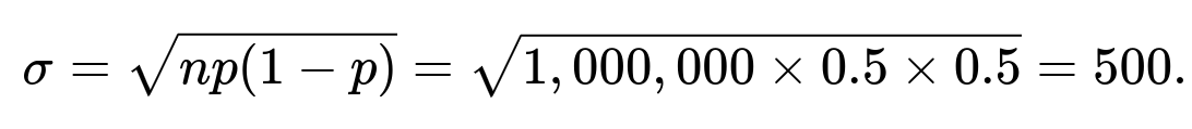
The difference from the mean 500,000 is 50,000, which is 100 standard deviations (50,000/500=100). This is astronomically unlikely for a fair coin.
Practical Implication With so many flips, the coin’s bias is detected with near certainty. The p-value is effectively zero for all practical purposes. This is far beyond typical significance thresholds.
Potential Pitfalls
If there were any data collection or measurement errors, they become extremely critical in such large-sample scenarios. Even tiny systematic errors can create large absolute deviations.
The coin or flipping mechanism might have changed partway through.
In such cases, discussing how large sample sizes can make even tiny biases unequivocally statistically significant reveals knowledge about how sample size drives the power of statistical tests.