
ML Interview Q Series: Hypothesis Testing for ML Classification: Navigating Type I and Type II Errors.
📚 Browse the full ML Interview series here.
Type I vs Type II Errors: Define Type I and Type II errors in hypothesis testing. Relate them to false positives and false negatives, and give an example of why understanding these errors is important in an ML context (for example, in detecting fraud or diagnosing illness).
Understanding Hypothesis Testing in Depth
Hypothesis testing is a fundamental procedure in statistics used to make inferences about a population based on a sample. The typical setup is that we have two hypotheses:
Null Hypothesis (often denoted as H0): This is usually the hypothesis of “no difference,” “no effect,” or “no change.” An example might be: “A patient does not have a certain illness,” or “This transaction is not fraudulent.”
Alternative Hypothesis (often denoted as H1 or Ha): This is the hypothesis that some effect, difference, or change exists. For instance: “A patient does have a certain illness,” or “This transaction is fraudulent.”
Once the data is collected, a test statistic is computed from the sample, and we use this test statistic to decide whether there is enough evidence to reject H0. In this process, two types of critical errors can occur, commonly referred to as Type I and Type II errors.
Type I Errors
Type I error occurs when H0 is actually true, but we mistakenly reject it. In a medical testing context, this corresponds to diagnosing someone as having a disease (rejecting the null of “healthy”) when that person is actually healthy. In other words, we saw evidence in the data that led us to incorrectly conclude something was there when it was not.
Relating Type I Errors to the ML notion of false positives: A Type I error in classical hypothesis testing is essentially a “false positive” in machine learning. For a fraud detection model, a false positive would be labeling a legitimate transaction as fraudulent.
Type II Errors
Type II error occurs when H0 is false, but we fail to reject it. In a medical testing example, this corresponds to diagnosing someone as healthy (accepting the null of “no disease”) when they do, in fact, have the disease.
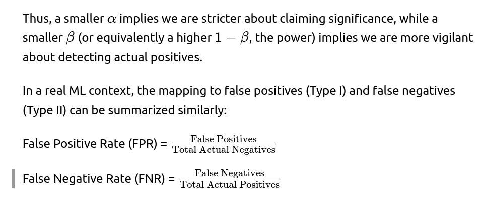
The probability of making a Type II error is denoted by β. The power of a test, often denoted by 1−β, measures the probability that the test correctly rejects H0 when H1 is indeed true. In practical machine learning, increasing the power means lowering the chance of missing an actual positive condition (like a real fraudulent transaction or a genuine case of illness).
Relating Type II Errors to the ML notion of false negatives: In machine learning terms, a Type II error is analogous to a “false negative.” For fraud detection, a false negative would be labeling a fraudulent transaction as “legitimate.”
Why It Matters in a Machine Learning Context
In real-world ML classification tasks such as fraud detection, spam email detection, or medical diagnosis, having insight into Type I and Type II errors is crucial for deciding on acceptable trade-offs:
If the cost of a Type I error is too high, we want to minimize false positives. For instance, in a medical screening test for a rare disease, you might not want to cause undue alarm or subject patients to expensive, invasive follow-up tests unless you are quite sure they are actually at risk.
If the cost of a Type II error is too high, we want to minimize false negatives. For example, in diagnosing a serious contagious illness, missing a truly infected patient could have dire consequences for both the patient and the public. Similarly, in a fraud detection system, failing to detect a fraudulent transaction might result in large financial losses.
Example: Fraud Detection
Consider a credit card company that wants to detect fraudulent transactions. H0 would be “The transaction is legitimate,” and H1 would be “The transaction is fraudulent.”
A Type I error (false positive) would mean flagging a legitimate transaction as fraud. This might annoy customers or cause some friction, but most credit card companies prefer a higher false-positive rate over a high false-negative rate, because they do not want fraudulent transactions to slip by.
A Type II error (false negative) would mean letting a fraudulent transaction go through without raising any alert. This is costly to the company and can undermine trust. Thus, many institutions lean toward a lower threshold for classifying transactions as fraudulent, accepting more false positives (Type I errors) to reduce false negatives (Type II errors).
Similar reasoning applies in medical diagnostics, spam detection, or any application where the balance between catching as many positives as possible and maintaining a reasonable false alarm rate has a big practical impact.
Deeper Discussion on the Trade-off
Choosing a decision threshold is a practical way to balance Type I vs. Type II errors in machine learning models. For example, suppose you have a model that outputs a continuous score indicating the likelihood of an instance (like a transaction or a patient) being positive (fraudulent or diseased). By adjusting that threshold, you can tilt the system toward catching more positives (reducing Type II errors) at the cost of also generating more false alarms (increasing Type I errors), or the other way around.
The exact choice of threshold often depends on domain-specific cost considerations. In some fields, a Type I error might be more damaging. In others, a Type II error is more damaging. Often, cost-sensitive learning is used to incorporate the real-world costs of each type of misclassification into the training process.
Example Code Snippet for Setting Threshold
Below is a simple Python snippet illustrating how you might adjust a threshold to control Type I and Type II errors in a fraud detection model. Suppose we have a model that outputs probabilities for each transaction. We want to test how Type I and Type II errors change with different thresholds:
import numpy as np

# Hypothetical ground truth labels: 1 = fraudulent, 0 = legitimate
y_true = np.array([0, 0, 1, 1, 0, 1, 0])

# Model predicted probabilities for being fraudulent
y_scores = np.array([0.1, 0.2, 0.7, 0.8, 0.05, 0.9, 0.4])

# Function to compute Type I and Type II errors at a given threshold
def compute_errors(y_true, y_scores, threshold):
    # Predict label based on threshold
    y_pred = (y_scores >= threshold).astype(int)

    # Type I error = false positives
    # Type II error = false negatives

    # False positives (Type I)
    fp = np.sum((y_true == 0) & (y_pred == 1))

    # False negatives (Type II)
    fn = np.sum((y_true == 1) & (y_pred == 0))

    return fp, fn

thresholds = [0.1, 0.3, 0.5, 0.7, 0.9]

for t in thresholds:
    fp, fn = compute_errors(y_true, y_scores, t)
    print(f"Threshold = {t}, Type I Errors (FP) = {fp}, Type II Errors (FN) = {fn}")
In such code, we systematically vary the threshold. As you increase the threshold, you will observe fewer false positives (Type I errors), but more false negatives (Type II errors). Lower thresholds typically reduce Type II errors but at the expense of more Type I errors.
Potential Follow-up Questions Begin Below.
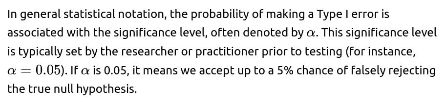
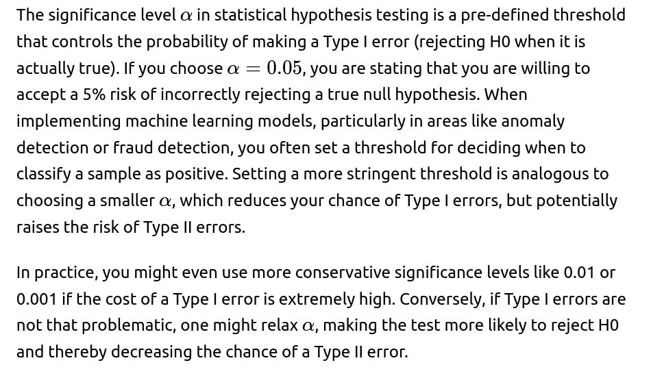
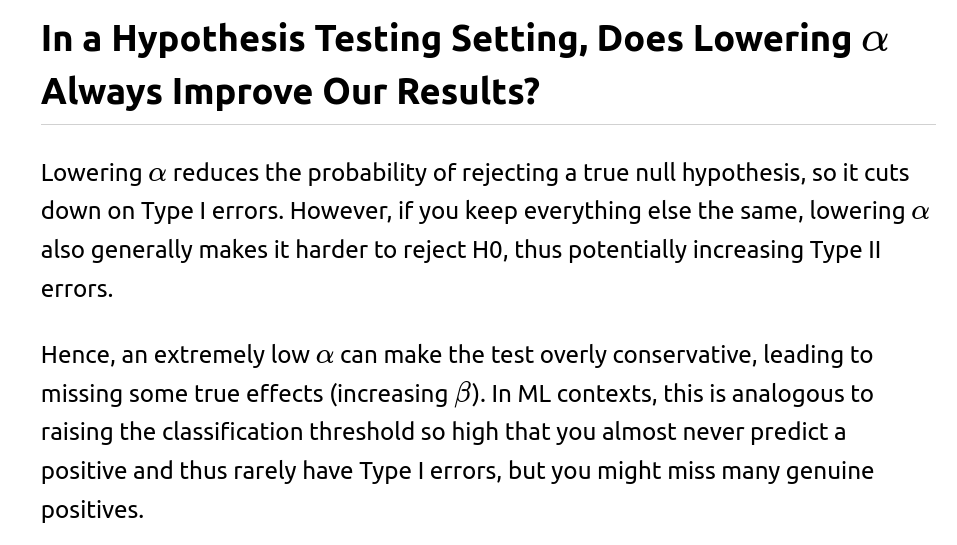
What Is the Role of the Significance Level αα in Controlling Type I Errors?
How Do Type I and Type II Errors Relate to Precision, Recall, and the ROC Curve?
Precision is the fraction of predicted positives that are truly positive. Recall (or sensitivity) is the fraction of true positives that are correctly identified as such.
Increasing recall tends to reduce Type II errors because you are catching more real positives. However, it may increase Type I errors in many cases, especially when the test or model tries to catch every possible positive. That can lead to more false alarms (false positives).
An ROC curve plots the true positive rate (TPR) against the false positive rate (FPR) at different classification thresholds. TPR is 1 minus the false negative rate, while FPR equals the false positive rate. By examining the ROC curve or the Precision-Recall curve, practitioners can choose an operating point that balances these errors based on the practical costs of false positives and false negatives.
Is There a Direct Way to Quantify and Trade Off Type I and Type II Errors in Machine Learning?
Yes. In many domains, you can design a cost function that incorporates the relative harm or cost of false positives and false negatives.
You can then optimize the model and its threshold to minimize the overall cost. For example, if a false negative is 10 times more costly than a false positive, you might shift the threshold downward to reduce Type II errors. Doing so will likely raise Type I errors, but overall cost might still be minimized if false negatives are truly more expensive.
Additionally, you can use metrics like the F-beta score. F-beta is a metric that weighs recall more than precision (or vice versa) depending on the chosen beta parameter. For instance, the F2 score weighs recall more heavily, thus penalizing Type II errors more strongly than Type I errors.
In Which Situations Would We Accept a Higher Rate of Type I Errors?
If the cost or risk of failing to detect actual positives is extremely high, we may allow for more Type I errors. For instance:
Cancer screening: Missing a patient who truly has cancer (Type II error) can be life-threatening. It is often viewed as acceptable to have more false alarms (Type I errors) because a follow-up diagnostic test can clarify whether the patient actually has cancer.
Critical system monitoring: Some high-stakes monitoring systems (like in aviation or nuclear facilities) would rather raise unnecessary alerts than fail to alert a truly hazardous condition.
Fraud detection: Many banks and financial institutions prefer to err on the side of flagging suspicious transactions (Type I errors) rather than letting fraudulent ones pass.
Could Class Imbalance Affect Type I and Type II Errors?
Yes. In problems like fraud detection or rare disease diagnosis, the percentage of actual positives (fraudulent transactions or diseased patients) is very low. A highly imbalanced dataset often means that a model can achieve high accuracy while barely catching any positives at all.
In such imbalanced settings, the risk of Type II errors (false negatives) can be substantially high if the model is not carefully calibrated. The model might frequently predict the majority class because that alone could yield good “overall accuracy,” even though it fails to detect the minority class. Techniques such as oversampling, undersampling, using class weights, and carefully tuning the threshold based on F1 or other specialized metrics can help mitigate imbalance-driven bias and keep track of both Type I and Type II errors in a fair manner.
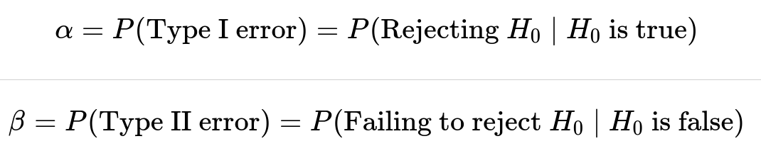
How Do We Formally Represent Type I and Type II Errors?
In standard statistical notation, we define:
What Are Some Common Techniques for Handling These Errors in Machine Learning?
Threshold tuning on model output probabilities is the primary lever. But more sophisticated techniques exist:
Calibrated Probability Estimates: Methods like Platt scaling or isotonic regression can help ensure your model’s predicted probabilities align with actual likelihoods, which makes threshold selection more meaningful.
Cost-Sensitive Learning: Incorporate custom loss functions or weighting schemes so that the model inherently pays more attention to the errors that are most costly in real life.
Resampling Techniques: For highly imbalanced data (leading to excessive Type II errors on the minority class), synthetic sampling (e.g., SMOTE) or undersampling can help reduce the model’s bias toward the majority class.
Ensemble Methods: By combining multiple models, you can often reduce variance and potentially reduce both Type I and Type II errors simultaneously, depending on how the ensemble is constructed and tuned.
Additional Considerations and Edge Cases
Real-world data often introduces additional complexity that can make error analysis and threshold setting more challenging. A few subtle scenarios include:
Shifting Data Distribution Over Time: In fraud detection, the types of fraud evolve quickly. The optimal threshold for balancing Type I vs. Type II errors might change over time, necessitating frequent re-training and recalibration of the model.
Different Regions of Feature Space Having Different Costs: Some groups of transactions might be more or less risky, and having a single threshold across all transactions might be sub-optimal. Segmenting the input space and applying different decision rules can sometimes reduce both types of errors in each segment.
Limited Labels or Data Quality Issues: In some cases, the ground truth for real positives might be incomplete or noisy. This can skew our understanding of Type I and Type II errors if we are not careful with data validation.
Below are some more potential follow-up questions with in-depth responses that might come up in a FANG-level interview setting.
How Do We Balance Type I and Type II Errors for a Final Model Deployed in Production?
Many production ML systems use a combination of business logic, domain expertise, and offline/online evaluation metrics:
Offline Analysis: You take historical labeled data, assess how changing a threshold impacts false positives and false negatives, and compute domain-relevant metrics like net cost, lost revenue, or patient well-being.
Domain Expert Review: In medical contexts, for instance, you might consult doctors or regulators to see how severe the risk is for each kind of error. In financial contexts, risk analysts or compliance officers may set guidelines.
A/B Testing or Phased Rollouts: Instead of immediately deploying a new threshold or model for the entire customer base, you might do a controlled rollout and monitor the real-world distribution of false positives and false negatives.
These strategies guide the final decision on the threshold or other design elements to ensure you achieve an optimal real-world trade-off.
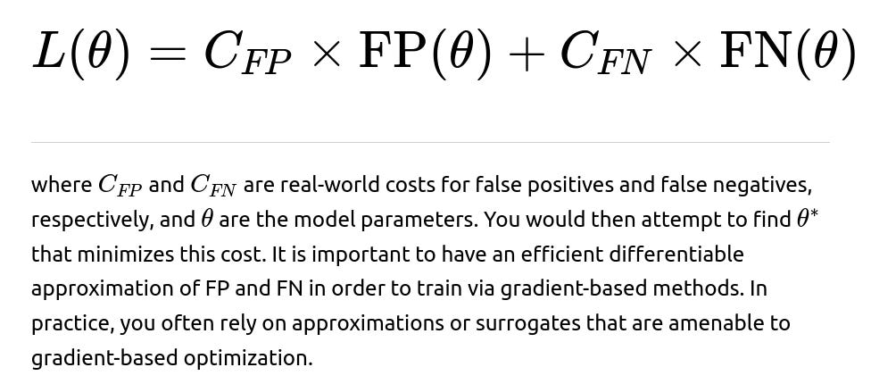
Could We Directly Optimize Type I and Type II Errors Using a Custom Loss Function in a Neural Network?
Yes, one approach is to define a loss function that includes terms for false positives and false negatives. In practice, many standard loss functions (such as cross-entropy) are not designed explicitly to control Type I or Type II errors but are indirectly related to them. However, in highly specialized applications, custom losses can be used.
For instance, you could create a function:
In Practice, Which Error Should We Prioritize Reducing?
It depends on domain context and the relative cost of each error:
In a disease diagnosis scenario, a false negative can be deadly, so Type II errors are often considered more critical.
In spam email detection, you do not want your important emails to go missing, so Type I errors (accidentally sending legitimate emails to spam) can have a high cost. Balancing them depends on user tolerance.
In a product recommendations system, the stakes for being wrong might be relatively low, so you might focus on overall user satisfaction metrics rather than strictly controlling Type I or Type II errors.
In short, domain context is essential. A strong ML practitioner always consults domain experts to quantify costs or at least weigh them qualitatively.
Summary of Key Points
Type I error (false positive) means rejecting a true null hypothesis, or labeling a negative sample as positive.
Type II error (false negative) means failing to reject a false null hypothesis, or labeling a positive sample as negative.
In ML classification tasks, Type I error corresponds to false positives, and Type II error corresponds to false negatives.
Balancing these errors in real-world scenarios depends heavily on the relative costs and risks associated with each misclassification.
The ultimate lesson is that understanding Type I and Type II errors is essential for effectively designing and deploying machine learning systems, especially in high-stakes domains where misclassifications have real-world consequences.
Below are additional follow-up questions
How Do You Estimate Type I and Type II Errors When You Have Incomplete Labels or Limited Ground Truth?
When data is only partially labeled (e.g., in fraud detection, you might only label certain confirmed fraud cases but not all legitimate transactions, or in medical diagnosis, some patients are not definitively diagnosed), direct measurement of false positives and false negatives becomes difficult. The fundamental challenge is that any transaction without a confirmed fraud label remains ambiguous.
One approach is to use methods such as active learning or targeted sampling to improve labeling in regions where mistakes (false positives or false negatives) are most likely to occur. For example, you can periodically audit a subset of unlabeled or low-confidence instances, get expert labels, and then estimate or correct for biases in your measured error rates.
Pitfall: If the sampling for labeling is not representative (e.g., an auditor only checks transactions above a certain risk score), the estimates of Type I or Type II errors might be overly optimistic or pessimistic. This makes it crucial to use a balanced or carefully stratified labeling strategy.
Edge case: In medical research, sometimes patients drop out of follow-up testing. If you only have labels for those who stayed in the study, you risk systematically missing false negatives among dropouts (people who tested negative initially but turned positive later). Handling such missing data typically requires specialized statistical methods (e.g., survival analysis approaches with censoring, or multiple imputation for missing data).
How Does Model Calibration Help Mitigate Type I and Type II Errors?
Model calibration involves adjusting a model’s output probabilities so that they accurately reflect the true likelihood of positive outcomes. Even if a model’s raw outputs can separate positives from negatives, these outputs might not align well with true probabilities. That misalignment can make it trickier to set an appropriate decision threshold.
By applying techniques like Platt scaling or isotonic regression, you can produce calibrated probabilities. Once these probabilities mirror real likelihoods, you can more reliably pick a threshold that optimizes for a desired balance between Type I and Type II errors.
Pitfall: Overfitting calibration data can happen if the calibration set is too small or not representative. A poorly calibrated model can increase one type of error if the calibration shifts the score distribution in a misleading way.
Edge case: In high-imbalance problems (e.g., very few positives), standard calibration might struggle unless you have enough positive examples to learn an accurate mapping. Advanced sampling or reweighting strategies might be necessary to ensure robust calibration.
How Do You Manage Type I and Type II Errors in an Online Setting With Distribution Shifts?
In an online system—say a real-time fraud detection or streaming anomaly detection—data distributions often evolve over time (a phenomenon known as concept drift). As the data drifts, models trained on older data may degrade in performance, leading to increased false positives or false negatives.
A typical strategy is to implement continuous monitoring of key metrics (like FPR, TPR, precision, recall) in production. When these metrics deviate significantly from their baseline, it may signal a shift in distribution that requires re-training or recalibrating the model.
Pitfall: A slow, gradual drift might go unnoticed until Type I or Type II errors accumulate substantially. Monitoring that only checks major deviations might react too late. A robust solution is to use techniques like rolling windows, time-decayed weighting of data, or anomaly detection specifically for the input feature space.
Edge case: In systems with cyclical or seasonal patterns, the model’s performance can degrade temporarily, then recover as the cycle repeats. Interpreting which changes are normal seasonal fluctuations vs. genuine distribution shifts is tricky, and your strategy might require domain insights to properly handle seasonal “drift.”
How Do Multiple Hypothesis Tests Affect Type I Error Rates in a Machine Learning Workflow?
When running multiple statistical hypothesis tests (for instance, testing multiple variants of a model or testing multiple metrics), the chance of at least one false positive (Type I error) grows if you do not correct for multiple comparisons.
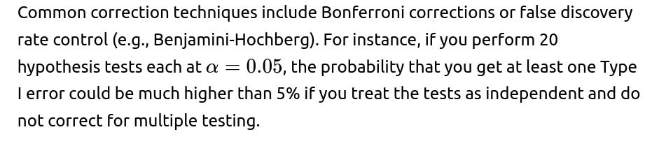
Pitfall: Overly strict corrections (like a naive Bonferroni) can become very conservative, potentially inflating Type II errors—meaning genuine effects might be missed.
Edge case: In large-scale model hyperparameter tuning, tens or hundreds of parameters might be tested. Without a proper correction, you can easily conclude that certain hyperparameters work “significantly better” due to random chance. This can lead to over-optimistic performance estimates that fail in real-world deployment.
How Do Type I and Type II Errors Translate to Decision Costs in a Real Business or Clinical Setting?
While false positives and false negatives are abstract statistics, real-world impact is measured in costs or consequences. For instance, in a bank:
A false positive on a fraud check might lead to an unnecessary call to a customer or a temporary card block. The direct cost is a customer service call and a possible inconvenience that could damage customer satisfaction.
A false negative would allow a fraudulent transaction to go through, leading to higher financial and reputational losses.
In a medical diagnosis:
A false positive might cause a patient to undergo unnecessary, potentially invasive testing (extra cost, emotional distress).
A false negative can lead to late detection of a serious disease, resulting in severe health consequences or even loss of life.
Pitfall: Many organizations only track one side of the error (e.g., the losses from letting fraud through) and do not properly quantify the “customer dissatisfaction cost.” This incomplete view can skew the threshold decision.
Edge case: The relative costs can vary dramatically across different segments or over time. For example, an extremely high-value transaction might be worth accepting a higher false-positive risk (manual review) compared to a small transaction. Handling these scenario-specific cost structures often requires dynamic thresholds or segment-based modeling.
How Do Type I and Type II Errors Manifest in Imbalanced Multiclass Problems?
When extending beyond binary classification to multiclass problems (e.g., diagnosing multiple diseases, or classifying multiple types of fraudulent behavior), you have multiple ways to generalize the concepts of false positives and false negatives. For each class, you can define a confusion matrix row by row or column by column, and then compute:
False positives for a specific class: cases incorrectly labeled as that class
False negatives for a specific class: cases that belong to that class but were labeled otherwise
Pitfall: A model might misclassify one minority class as another minority class. Tracking a global Type I or Type II error can mask which specific class is being misclassified. This is why analyzing the per-class confusion matrix is crucial.
Edge case: Some real-world settings have more than two classes, but the cost structure is more important for certain classes. For instance, you might have “legitimate transaction,” “friendly fraud,” “organized fraud,” and “technical error” as multiple classes. The real cost might be highest for missing organized fraud. Hence, you might accept more confusion among the other classes just to reduce false negatives on the organized fraud class.
How Do Type I and Type II Errors Play Out in Reinforcement Learning Settings?
Although reinforcement learning (RL) typically focuses on maximizing long-term reward rather than minimizing classification error, the concept of Type I and Type II errors can still arise in sub-problems within RL. For instance, in a policy that detects a rare event and triggers a certain action, a false positive could mean an unnecessary action, while a false negative could mean failing to take a crucial action.
One challenge is that, in RL, feedback (rewards) about a positive or negative action may be delayed, partial, or noisy. This partial feedback complicates the direct measurement of false positives or false negatives in each step.
Pitfall: Overfitting to short-term rewards might inadvertently increase either Type I or Type II errors in the long run. For instance, the agent might take too many “safe actions” to avoid penalties in the short term, inadvertently generating excessive false positives.
Edge case: In high-stakes RL scenarios (e.g., robotics, self-driving cars), a single false negative (failing to detect an obstacle) can be catastrophic. One approach is to incorporate risk-sensitive or safety-oriented methods that explicitly penalize dangerous false negatives more heavily than false positives.
Could a Model Perform Well on Average Yet Have High Type I or Type II Errors in Specific Subgroups?
Yes. This is closely related to fairness and bias issues. A model might yield overall acceptable false positive and false negative rates but perform poorly for certain protected groups. This translates to substantial Type I or Type II error disparities among demographic subgroups.
Pitfall: Relying solely on global error metrics can mask these subgroup-specific problems, leading to unfair or even illegal discrimination in domains such as hiring, lending, or medical diagnosis.
Edge case: If a certain subgroup is underrepresented in the training data, the model might systematically produce more false negatives for that group. Addressing this often requires additional data collection, reweighting, or specialized fairness constraints (e.g., equal opportunity constraints to ensure balanced false negative rates across groups).
How Can You Systematically Explore the Trade-off Curve Between Type I and Type II Errors in Practice?
One common method is to plot a Precision-Recall curve or an ROC curve across various thresholds. From these plots, you can visualize how the true positive rate and false positive rate change as you shift the classification boundary.
You then overlay business or clinical constraints on top of that curve. For example, if you know that surpassing a certain false positive rate is extremely costly, you look for a threshold that keeps FPR below that limit while trying to maximize TPR.
Pitfall: In highly imbalanced datasets, the ROC curve can be overly optimistic, and the Precision-Recall curve often presents a clearer picture of performance for the positive class.
Edge case: If the positive class is extremely rare (e.g., 0.1% of the data), even small absolute changes in the false positive rate can lead to a large relative number of false positives. You might need to zoom in on a very specific region of the curve (a high-precision zone) to find a practical operating point.
How Can Active Learning Strategies Help Reduce Type I and Type II Errors Over Time?
Active learning focuses on selectively querying the most informative or uncertain samples for labeling. The goal is to improve the model using fewer labeled samples, which is especially valuable in cases where labeling is costly (e.g., needing expert verification for fraud or medical data).
By directing labeling efforts at samples near the decision boundary, active learning can help the model refine that boundary, reducing both false positives and false negatives in the region that matters most for your application.
Pitfall: If active learning is solely driven by model uncertainty, the model might repeatedly sample from certain feature space regions and overlook rare but critical outlier patterns—thus failing to reduce false negatives in those outlier segments.
Edge case: In an online environment, combining active learning with real-time feedback from domain experts requires a robust infrastructure for continuously updating the training set and re-deploying the model, which can be technically complex and prone to distribution shifts.
How Do We Incorporate Human-in-the-Loop Systems to Manage Type I and Type II Errors?
In some high-stakes or high-cost-of-failure domains, a typical workflow is to have a model provide initial screening, then route ambiguous or high-risk cases to a human expert for review. The human can override the model’s prediction if needed. This approach can lower overall false negatives (since the expert can catch subtle positives) without exploding the false positive rate for all instances.
Pitfall: If the system floods human reviewers with too many cases (due to a high false positive rate), reviewers might become fatigued or complacent. Their error rate could rise because they start to trust the model’s predictions too often.
Edge case: Over time, human reviewers might adapt to the model’s blind spots. They might devote more time to particular scenarios the model is prone to misclassify. This co-adaptation can be beneficial but also risky if not tracked. If the model’s distribution changes, the human reviewers might need new training or updated knowledge about the model’s new failure modes.
How Do You Monitor Type I and Type II Errors in Post-Deployment, Real-World Systems?
It is critical to define a feedback loop. For example, in a fraud detection scenario, real fraud might be discovered days or weeks after the transaction. That delayed label has to be integrated back into the system to re-measure false negatives (transactions flagged as legitimate that turned out fraudulent). Similarly, legitimate transactions that were flagged and reversed must be accounted for as false positives.
Pitfall: In some contexts, it is impossible to get perfect ground truth for negatives (e.g., a transaction that was never proven fraudulent might simply have been unobserved or not yet discovered). This incomplete feedback can bias your error estimates.
Edge case: After a user is falsely flagged multiple times, they might change their behavior (e.g., they use a different payment method), or they might churn from the system entirely, so you lose the ability to track their subsequent activity. This phenomenon is known as “selective labels” or “label leakage,” where the process of flagging or intervening changes the data distribution and complicates error measurement.
What Is the Difference Between a Statistical Confidence Interval and the Probability of a Type I Error?
A statistical confidence interval (for example, a 95% confidence interval around a mean) indicates the range within which the true parameter (like a population mean) is likely to lie given the observed data. It does not directly speak to the probability of incorrectly rejecting H0 in hypothesis testing.
Pitfall: Conflating these concepts can cause confusion. For instance, having a confidence interval for a parameter that barely excludes zero does not always mean the Type I error rate is 5%; it means that if you were to repeat the experiment many times, about 95% of the calculated intervals would contain the true parameter.
Edge case: In ML experiments, we often estimate model performance (e.g., accuracy, F1-score) with confidence intervals derived from cross-validation. But those intervals do not guarantee that if your model outperforms baseline by a certain margin, the probability that you’re seeing a “lucky fluke” is below some threshold. They are a measure of variability, not strictly the probability of a Type I error in a classical hypothesis-testing sense.
How Does the Prevalence of the Positive Class Affect Type I and Type II Errors?
Prevalence is the base rate of the positive class in the population (e.g., the proportion of fraudulent transactions, or the rate of a disease in a patient population). If prevalence is very low, even a small false positive rate can result in many more false positives than true positives. Conversely, if the prevalence is high, even a moderate false negative rate can miss a lot of actual positives.
Pitfall: Focusing on accuracy alone can be misleading, especially if the prevalence is skewed. A trivial model predicting every instance as negative might achieve high accuracy but fail catastrophically in terms of false negatives.
Edge case: In some adaptive systems, the prevalence can change after the system is deployed. For example, a successful fraud detection system might discourage fraudsters from certain tactics, causing the fraction of certain types of fraud to drop. If the model is not updated, it might continue to produce false positives at the same rate, even though actual fraud patterns are shifting.
How Can External Constraints or Regulations Affect the Acceptance of Type I and Type II Errors?
In many industries—like healthcare, finance, or autonomous vehicles—regulatory bodies set rules or guidelines for acceptable levels of misclassifications. For instance, a regulatory agency might require medical tests to have a minimum sensitivity (i.e., TPR) to ensure that few diseased patients are missed. This effectively puts an upper bound on Type II errors.
Pitfall: If you push sensitivity extremely high to meet regulations, you might inadvertently raise Type I errors and produce an unmanageably high false-positive workload.
Edge case: Regulations can also mandate that you cannot discriminate across demographic groups. You might have to demonstrate that false negatives (Type II) for one group are not significantly higher than for another. This can lead to more complex objective functions where you try to optimize overall performance subject to fairness constraints.
How Do We Diagnose Whether Our Model Is Suffering More From Type I or Type II Errors Without a Balanced Dataset?
One practical approach is to create a confusion matrix on a test set that has known positives and negatives. If the dataset is imbalanced, you can do one of the following:
Use stratified sampling to maintain the same ratio of positives to negatives that appears in the real world, then measure false positives and false negatives.
Oversample positives or undersample negatives to get a balanced or near-balanced test set, calculate errors, and then adjust the metrics back to real-world prevalence.
You also can measure metrics like precision, recall, and specificity:
High recall but low precision often implies more Type I errors.
High precision but low recall often implies more Type II errors.
Pitfall: If you artificially balance the test set (e.g., 50% positives, 50% negatives) but do not correct the metrics accordingly, your false positive rate in real-world conditions might be underestimated.
Edge case: In some domains, the notion of “positive” might be fluid or ambiguous (e.g., borderline medical conditions or suspicious transactions with partial evidence). In these cases, even labeling the test data can involve subjective judgments, adding noise to the measured Type I and Type II errors.
How Do You Evaluate and Mitigate the Long-Term Impact of Repeated False Positives or False Negatives on User Behavior?
In repeated-use scenarios (e.g., spam email filtering, ongoing medical screenings), repeated false positives can cause users to lose trust in the system, while repeated false negatives can cause them to overlook genuine issues. Therefore, you must consider the cumulative or compound effects.
Strategies to mitigate long-term impact include:
Gradual threshold tuning and user feedback loops
Personalized or context-aware thresholds that learn from each user’s behavior
Explanations to the user when the system flags something as suspicious or healthy, helping them understand why
Pitfall: Users might adapt in unpredictable ways. For example, if the system frequently flags legitimate emails as spam, users might stop checking their spam folder altogether, increasing the chance of missing actual spam or incorrectly flagged emails.
Edge case: In critical domains, a single false negative might be catastrophic (e.g., a patient not receiving an urgent medical alert). In that scenario, you might allow more false positives over the short term until you have enough data to reliably reduce them without increasing the risk of missed positives.
How Should We Handle Situations Where the Null Hypothesis Is Not the “No Event” Condition?
In classical hypothesis testing, we often treat the null as “no effect” or “no difference.” However, in certain real-world cases (like a new product launch or new medical treatment), the null might be that the new treatment is equally effective as the old one, and the alternative is that it’s better.
Type I error then represents concluding the new treatment is better when it is not, and Type II error is concluding it’s not better when it actually is. While the mapping to “false positive” and “false negative” remains conceptually similar, the practical interpretation can change.
Pitfall: In medical research, incorrectly concluding that a new drug is better (Type I error) can lead to widespread adoption of an ineffective or harmful drug. Alternatively, failing to adopt a beneficial drug (Type II error) can have significant missed-benefit consequences for patients.
Edge case: Some experimental designs reverse the roles of H0 and H1 (e.g., non-inferiority trials in pharmaceuticals). The nature of Type I and Type II errors might be framed differently, and ensuring the correct interpretation is crucial to avoid misapplication of hypothesis testing in practice.
How Do You Communicate Type I and Type II Errors to Non-Technical Stakeholders?
Conveying the concept of false positives and false negatives in plain language is critical to get buy-in from domain experts, executives, or regulatory agencies. One method is using scenario-based examples:
“Out of 1,000 legitimate transactions, we accidentally flagged 20 as fraud (false positives). This might upset those 20 customers.”
“Out of 100 fraudulent transactions, we failed to catch 10 (false negatives). This led to direct financial losses.”
Pitfall: Merely reporting “we have a 2% false-positive rate” can be meaningless without context on the total volume. Non-technical stakeholders might misinterpret or trivialize the implications.
Edge case: In certain fields, key stakeholders might only care about the worst-case scenario. For example, a hospital might ask, “What if that false negative is a life-threatening disease?” So you might need to provide not just average metrics but also risk-based breakdowns of the most severe outcomes.
How Do Type I and Type II Errors Arise in Generative or Self-Supervised Learning Tasks?
In generative models (e.g., for text generation, image synthesis), the concepts of Type I and Type II errors can appear in evaluation sub-problems. For instance, a “false positive” might be generating content that is classified as realistic or correct when it is not. A “false negative” might be failing to generate a valid concept that should be possible under the data distribution.
Pitfall: Subjective evaluations are common in generative tasks (like the realism of generated images or the fluency of generated text). Standard definitions of Type I and Type II errors become blurred if the ground truth is not strictly binary (e.g., something can be partially correct).
Edge case: In text generation, certain tasks have clearly defined constraints (like grammar rules or known facts). The generative model might appear to follow them but occasionally produce “hallucinations,” effectively a false positive (the model claims a statement is valid when it is incorrect). If the environment is zero-sum (like misinformation detection), these errors are costly and need specialized mitigations.
How Do We Use Confidence Intervals for Model Metrics (e.g., Accuracy, AUC) to Infer Possible Type I or Type II Error Bounds?
While confidence intervals for metrics like accuracy or AUC provide a sense of statistical variability, they do not directly give you false-positive or false-negative rates under all thresholds. However, you can sample from the distribution of predictions (via bootstrap or cross-validation) to derive intervals for FPR and FNR at a given threshold.
Pitfall: Relying on a single test set and computing a single point estimate for FPR or FNR can be misleading—especially if the test set is not large or is unrepresentative.
Edge case: If you’re dealing with extremely rare events, the confidence intervals for FPR or FNR can become quite wide unless you have a massive sample of data. This can complicate decisions about threshold tuning if you do not have enough examples of the positive class to get a stable estimate.
How Could Emerging Privacy Restrictions (e.g., GDPR) Influence Measurement of Type I and Type II Errors?
Laws like GDPR can restrict data retention, making it harder to track outcomes and measure errors over time. For instance, if you must delete user data after a certain period, you might lose the ability to verify whether older predictions were false positives or false negatives. Additionally, obtaining ground-truth labels might require explicit user consent, limiting your labeled dataset.
Pitfall: If you cannot store certain personally identifiable information, you might lack the necessary contextual features for accurate classification. This could push up either Type I or Type II errors, depending on how critical those features were.
Edge case: The “right to be forgotten” could erase records you need to detect repeat fraudulent behaviors. The system might treat a known fraudster as a fresh user, inadvertently repeating the same Type I or Type II errors. Techniques like anonymization or secure hashing can partially mitigate these problems but need to comply strictly with privacy regulations.
How Do Type I and Type II Errors Interact With Interpretability in Machine Learning?
Highly complex models (e.g., large neural networks) can be difficult to interpret, making it challenging to explain why a particular sample was classified as positive or negative. If stakeholders cannot understand why a system produced false positives or false negatives, they may mistrust or reject the model altogether.
Pitfall: Even if a model has good overall performance, its “black-box” nature might obscure systematic biases or pockets of high false-negative rates in certain conditions. This can be especially problematic in regulated industries where explainability is required.
Edge case: Methods like LIME or SHAP provide local explanations for model predictions, potentially revealing consistent reasons behind false positives or false negatives (e.g., certain keywords or features). However, these explanation methods have their own limitations, and a misleading explanation can itself cause stakeholders to misjudge the severity of Type I or Type II errors.
How Do Type I and Type II Errors Affect the Design of Manual Overrides or Fallback Mechanisms?
Many production systems include fallback rules—manual or heuristic-based checks—that override model decisions. For example, a credit card might have a rule: “If the transaction amount is over $10,000 from a new user, automatically flag for review regardless of model score.” Such rules aim to mitigate high-stakes false negatives.
Pitfall: Over-reliance on fallback rules can overshadow the model’s benefits if the fallback triggers too often. You might end up with excessive false positives, negating the efficiency gains of automation.
Edge case: If the fallback rules are derived from older patterns (e.g., historical insights about how fraud was done years ago), they might cause a mismatch with modern patterns. The system can end up with unpredictable interplay: the model might classify something as legitimate, but the fallback flags it anyway for a manual check—leading to user frustration and potential duplication of work.
How Does Early Stopping or Model Regularization Influence Type I and Type II Errors?
In supervised learning, you typically split data into training and validation sets, and you might apply early stopping to prevent overfitting. Overfitting often manifests as a model that appears to reduce both false positives and false negatives on the training set but performs poorly on validation or test data.
With proper regularization and early stopping, you often get better generalization. This reduces both Type I and Type II errors on unseen data compared to an overfit model. However, the exact effect on each error type depends on the nature of the overfitting.
Pitfall: If you over-regularize or stop too early, the model might be underfitting, which could elevate both false positives and false negatives (or shift them in unpredictable ways).
Edge case: In some specialized tasks, a slight overfit might be acceptable if you’re trying to minimize false negatives above all else. For instance, in a medical screening for a deadly disease, if slight overfitting means fewer missed positives, the trade-off might be worthwhile—though you should still keep an eye on generalization performance in real-world settings.
How Do We Quantify the Uncertainty in Our Estimates of Type I and Type II Errors?
Because all measurements of false positives and false negatives are sample-based, we can compute confidence intervals or credible intervals (in a Bayesian context) around these estimates. A typical frequentist approach might apply a binomial proportion confidence interval for FPR or FNR.
Pitfall: A naive confidence interval formula might not account for correlation between samples or for the model’s possible overfit to your data split. You might need advanced bootstrap methods or cross-validation to get a more robust interval.
Edge case: In real-time streaming data with autocorrelation (e.g., repeated transactions from the same user), standard binomial assumptions can be violated. FPR or FNR estimates might require specialized time-series or hierarchical modeling approaches to capture the correlation across events from the same source.
How Do You Handle a Scenario Where Type I or Type II Error Definitions Are Not Clear-Cut?
Some problems don’t have a clean boundary between positive and negative, such as detecting “interesting” or “useful” content in a recommendation system. One user’s interesting content might be uninteresting to another. In these subjective domains, the concept of a “true” positive vs. negative can be fuzzy.
Pitfall: If you force a binary ground truth label (“interesting” vs. “not interesting”) based on minimal feedback, you might artificially inflate either false positives or false negatives. This can degrade user experience over time.
Edge case: A more nuanced approach might track user engagement signals (e.g., watch time, likes, shares) rather than a binary classification. In this setting, false positives and false negatives become tied to user satisfaction metrics, requiring careful experimental design (like A/B testing) to gauge real-world impact.
How Do Oversampling or Undersampling Techniques Affect Type I and Type II Error Rates?
When dealing with a highly imbalanced dataset, oversampling the positive class (e.g., SMOTE) or undersampling the negative class can help the model train on a more balanced view of data. This often reduces false negatives (Type II errors) for the minority class. However, if the oversampling introduces too many synthetic examples that are not representative, or if undersampling discards too many negative examples, the model might learn boundaries that are not optimal, possibly inflating false positives (Type I errors).
Pitfall: SMOTE or random oversampling might replicate rare edge cases or generate synthetic samples that do not accurately reflect real-world data, leading to over-optimistic estimates of model performance.
Edge case: If your negative class is extremely large (e.g., 10 million examples) and your positive class is very small (1,000 examples), random undersampling can cause you to lose a vast amount of potentially valuable negative data. A more nuanced approach (stratified or cluster-based undersampling) might be necessary to preserve a good representation of the negative class distribution.
Are There Situations Where You’d Actively Prefer to Increase a Certain Error Type?
Yes, if your domain or product requirements favor one error type due to cost or strategy considerations. For example, in marketing lead qualification, you might prefer to err on the side of false positives—i.e., reaching out to some leads who are not actually interested—rather than missing out on valuable leads (false negatives).
Pitfall: Overly aggressive outreach can annoy potential customers who are labeled as leads but have no interest, possibly damaging your brand.
Edge case: In a triage system for mental health crises, you might prefer to route borderline cases to care rather than risk missing a serious crisis. In that scenario, you deliberately allow more Type I errors (false positives) for the sake of reducing Type II errors (false negatives) to a minimal level.
How Do We Handle Situations Where the Ground Truth Labels Themselves Have Error or Noise?
In some datasets, even the “true” labels are uncertain. For example, in medical imaging, different radiologists might disagree on whether a lesion is benign or malignant. This label noise can confuse the model, leading to an inflated estimate of both false positives and false negatives (some “errors” might just reflect label disagreement).
Pitfall: If you treat noisy labels as gospel, you might train a model that attempts to replicate the labeling inconsistencies. This can distort your measurement of Type I and Type II errors, because you are partially capturing label noise rather than genuine misclassifications.
Edge case: Methods for learning with noisy labels (like using a confusion matrix for annotators or employing a consensus approach) can mitigate the problem. However, if the label disagreement itself is high, it becomes difficult to define a precise ground truth. In such a scenario, you might measure inter-annotator agreement as a reference baseline for your model’s performance.
How Does the Concept of Type III Error Fit Into This Discussion?
A Type III error is sometimes informally mentioned in statistical literature as an error where you correctly reject H0 for the wrong reason, or you correctly reject H0 but answer a different question than what you intended to test. In ML contexts, you could think of it as the model making a “correct” classification for a spurious or unrelated reason (like overfitting to an artifact).
While less formally recognized than Type I or Type II, it underscores the importance of verifying that your model’s reasoning generalizes. If your model is correct for the “wrong reason,” it might fail badly under slightly changed conditions.
Pitfall: Relying purely on performance metrics can hide the fact that your model is using spurious correlations to achieve good accuracy on the training or test sets. This can lead to unexpected spikes in false positives or false negatives when the distribution changes.
Edge case: In image recognition tasks, a model might learn to detect a label from background details rather than the object of interest. During deployment (with different backgrounds), it suddenly exhibits high false negative rates for images it previously handled well in test data.
How Do You Implement Hierarchical Classification to Reduce Certain Error Types?
A hierarchical classification approach breaks down a complex classification decision into stages. For example, you can first decide if a transaction is suspicious or not. If suspicious, you pass it to a more specialized model or rule-based system to determine whether it is truly fraudulent. This two-stage approach can help refine the boundary.
Pitfall: If the first stage is too aggressive, you might flood the second stage with too many false positives, overloading resources. If it’s too lenient, you risk too many false negatives skipping detailed scrutiny.
Edge case: In medical diagnostics, you might have a preliminary screening test (which can afford to be highly sensitive, i.e., few false negatives) followed by a confirmatory test (which aims to reduce false positives). The overall result is that Type I or Type II error is more tightly controlled across the pipeline.
How Might an Adversary Exploit Knowledge of Your System’s False Positive or False Negative Rates?
In adversarial settings (fraud, spam, cybersecurity), attackers might deliberately craft inputs that exploit your system’s weaknesses. If they realize the system is tuned to avoid false positives at all costs, they might attempt borderline behaviors that slip under the threshold.
Pitfall: If you publicly disclose that your system has a very low tolerance for false positives, adversaries might guess that your threshold is set high, so they can operate in a region just below that threshold to evade detection (increasing Type II errors).
Edge case: A dynamic adversary might run test queries to see when they trigger a positive. This feedback loop lets them calibrate their own strategy. The interplay of Type I/Type II errors becomes an arms race, where each side attempts to outmaneuver the other’s boundary.