ML Interview Q Series: Identifying a Double-Tailed Coin Using Bayesian Inference After Consecutive Tails

Browse all the Probability Interview Questions here.

Suppose you have two coins: one is fair (heads on one side, tails on the other) and the other is biased (both sides are tails). You randomly pick one of these coins, flip it five times, and all five results are tails. What is the probability that you are flipping the double-tailed coin?

Short Compact solution

Comprehensive Explanation

Bayes’ theorem helps us update our belief in which coin we have after we observe the outcome of flipping it multiple times. Initially, we have no reason to favor one coin over the other, so the prior probabilities for choosing either coin are both 1/2. After flipping the chosen coin five times and seeing all tails, the likelihood of that event under each coin type becomes crucial in updating our belief.

Bayes’ theorem in its simplest form for our problem can be written as:

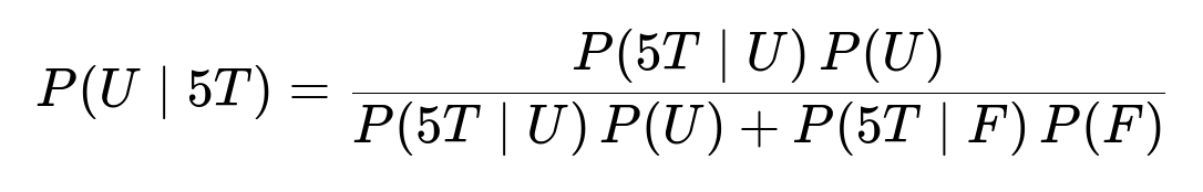
Here:

• ( P(U \mid 5T) ) is the probability that we are using the unfair coin given that we observed five tails.

• ( P(5T \mid U) ) is the probability of getting five tails given the coin is unfair (equal to 1).

• ( P(5T \mid F) ) is the probability of getting five tails given the coin is fair (equal to (1/32)).

• ( P(U) ) is the prior probability of having selected the unfair coin (1/2).

• ( P(F) ) is the prior probability of having selected the fair coin (also 1/2).

Substituting the values:

Hence, after seeing five tails in a row, we have a 97% chance that we picked the double-tailed coin.

The intuition is straightforward: although a fair coin can come up tails five times in a row, it is relatively unlikely. Meanwhile, for the double-tailed coin, seeing tails five times is not surprising at all. This disparity in likelihood drives the posterior probability strongly toward the coin with two tails.

Follow-up Question: Why Is the Prior Probability 1/2?

If you do not have additional information about which coin is more likely to be picked, the natural assumption is that each coin is equally likely to be chosen. This gives each coin a prior probability of 1/2. In more general cases, you might have different priors based on domain knowledge or empirical frequency (for example, if you know that one coin is more likely to appear in a random draw). Then you would adjust the prior probabilities accordingly.

Follow-up Question: What if You Flip the Coin (n) Times?

If you generalize to (n) flips, you would see tails on all (n) flips. For the fair coin, the probability of (n) consecutive tails is (1/2^n). For the double-tailed coin, it’s still 1. Using Bayes’ theorem, the formula for the posterior probability of having the unfair coin after (n) tails in a row would be:

As (n) increases, (1/2^n) becomes very small, so the posterior probability that you have the double-tailed coin grows even closer to 1.

Follow-up Question: Could a Fair Coin Legitimately Produce Five Tails in a Row?

Yes, there is a legitimate (though relatively small) chance that a fair coin will do so. The likelihood of 5 consecutive tails for a fair coin is 1/32, which is not extremely tiny but is still significantly smaller compared to the certainty of a double-tailed coin producing tails every time. This difference in likelihood is why we update our belief so strongly in favor of the double-tailed coin.

Follow-up Question: How Does This Relate to Bayesian Inference in General?

This question illustrates the essence of Bayesian inference: we start with a prior belief (each coin is equally likely), we collect evidence (five tails in a row), and then we update our belief in light of the evidence. The posterior probability quantifies our new degree of belief about which coin we have. This process reflects a key principle in machine learning and statistics: models are updated as new information arrives, improving our understanding or prediction in the face of uncertainty.

Follow-up Question: Implementation in Python

A simple Python snippet to compute this probability could look like this:

def posterior_probability(n_tails, prior_unfair=0.5):
    import math

    # Probability of n_tails with unfair coin (double-tailed) is always 1
    prob_n_tails_unfair = 1.0

    # Probability of n_tails with fair coin
    prob_n_tails_fair = (0.5 ** n_tails)

    # Compute posterior with Bayes' theorem
    numerator = prob_n_tails_unfair * prior_unfair
    denominator = numerator + prob_n_tails_fair * (1 - prior_unfair)
    return numerator / denominator

print(posterior_probability(n_tails=5))

When you run this, you should see a result close to 0.97 for five consecutive tails.

Follow-up Question: What if the “Fair” Coin Is Actually Biased?

If the fair coin is not truly fair, and instead has some unknown probability (p) of landing tails, then you would replace the term (1/2^5) with (p^5). The same Bayes’ logic applies, but you would need that (p) value (or a prior for (p)) to compute the likelihood of five consecutive tails. If (p) were close to 0.5, the result would still be similar, but if (p) were significantly larger (say 0.7 or 0.8 for tails), the posterior probabilities would shift differently. This underscores that Bayesian updating always depends on how we model the likelihood of the observed data under each hypothesis.

---

Below are additional follow-up questions

What if we change the question to predicting the outcome of the next flip rather than identifying the coin?

In a Bayesian framework, once we observe five consecutive tails, we update our belief about which coin we likely have. If our question changes to, “What is the probability the next flip lands on tails?” rather than “Which coin do we likely have?”, we can answer by computing a posterior predictive probability. Concretely:

• We have two hypotheses: unfair coin (double-tailed), and fair coin.

• After seeing five tails in a row, the posterior probability of having the unfair coin is about 0.97 (from the previous derivation).

• The posterior probability of having the fair coin is about 0.03.

To predict the next flip, we take a weighted average of the probability of tails under each hypothesis:

• Probability of tails given unfair coin: 1.

• Probability of tails given fair coin: 0.5.

Thus, the probability of tails on the next flip is:

So there is roughly a 98.5% chance the next flip is tails. Pitfall: If someone just said “It’s the unfair coin with 97% probability,” they might incorrectly conclude there is a 100% chance of tails on the next flip. The subtlety is that we still have a 3% chance we might have the fair coin, and hence only a 50% chance of tails in that case.

How might one handle the scenario where the “unfair” coin has a slightly higher probability of tails but not necessarily 100%?

In a more general setting, the “unfair” coin might not always land tails but could have a bias ( p ) strictly between 0.5 and 1. In that case:

1. The probability of (n) tails in a row when using the unfair coin is ( p^n ).

2. For the fair coin, it remains ( (0.5)^n ).

3. Bayes’ rule still applies. Instead of using 1 as the likelihood for “unfair” coin tails, we use ( p^n ).

Edge Case: If ( p ) is unknown, we might introduce a Beta prior over ( p ) and use a Bayesian updating approach to infer it. This complicates the problem, turning it into a problem of inferring both which coin we have and the parameter ( p ) itself.

Pitfall: Failing to model the possibility that the unfair coin might sometimes show heads could lead us to overly strong posterior beliefs in the event we happen to see an unlikely outcome (such as a head) after the initial five tails.

How does the sample size of five flips affect the strength of our Bayesian update?

Observing only five flips gives limited evidence, though they are still quite informative. If we observe tails more times (for instance, 10 or 20 flips), the posterior probability of the double-tailed coin would grow even larger. Conversely, if we see a single head in our flips, the probability of having the double-tailed coin collapses to zero immediately (assuming a perfectly double-tailed coin).

Pitfall: Stopping too soon can mislead. If we do only one or two flips, the evidence might not be strong enough to favor the double-tailed coin. For example, if we see just one tail, that is not particularly surprising for a fair coin, so it does not strongly update our posterior.

Edge Case: If someone repeated this experiment many times, frequent short series of flips might produce a spurious conclusion if we only occasionally see a run of tails. In real-world scenarios, collecting more data is almost always better for robust inference.

How would a frequentist approach address the probability that we selected the unfair coin?

A strict frequentist approach generally does not speak directly about the probability of hypotheses (i.e., “the probability that this coin is unfair”) because frequentist inference interprets probability as limiting frequencies of outcomes rather than degrees of belief in hypotheses. Typically, a frequentist might perform a hypothesis test. For example:

1. Null hypothesis ((H_0)): The coin is fair.

2. Alternative hypothesis ((H_1)): The coin is not fair.

They might compute the p-value that a fair coin would produce the observed outcome (five tails in a row). This p-value is ( (1/2)^5 = 1/32 = 0.03125 ). If the p-value is below a chosen significance level (e.g., 0.05), they would reject (H_0). But this still does not translate directly to “the probability is 97% that we have the unfair coin.” That is a Bayesian concept.

Edge Case: If we have multiple flips or even multiple coins, frequentist approaches might require repeated sampling and more complex hypothesis testing.

Pitfall: Interpreting the p-value as the probability of the hypothesis being false is a common misunderstanding. In frequentist terms, the p-value is the probability of the observed outcome (or more extreme) assuming the null is true, not the probability that the null is true itself.

Could we incorporate a cost function to handle different penalties for wrong decisions?

Sometimes we might prefer to err on the side of a particular decision if the cost of being wrong is higher. For instance, if picking the wrong coin leads to large financial loss or safety issues, we might need to incorporate a cost or utility function:

• Let ( C(\text{pick fair}|\text{unfair coin}) ) represent the cost of deciding we have a fair coin when in fact it is unfair.

• Let ( C(\text{pick unfair}|\text{fair coin}) ) represent the cost of the opposite incorrect decision.

In Bayesian decision theory, we compute not just posterior probabilities but also expected utilities. The best decision is the one that maximizes expected utility (or equivalently minimizes expected cost).

Edge Case: If ( C(\text{pick fair}|\text{unfair coin}) ) is extremely high, we might conclude that even a moderate posterior probability of the unfair coin is enough to label it as unfair.

Pitfall: Overlooking the cost structure can lead to suboptimal real-world decisions. Just because the posterior probability is not extremely high (e.g., 70%–80%), one might still choose a conservative decision if the penalty for being wrong is large.

How do practical issues like coin damage or an extremely small sample size affect our inference?

Real-world coins can get damaged, worn, or not be perfectly symmetrical, creating slight biases. If either coin is damaged, it might behave unexpectedly.

1. A damaged fair coin might have a slightly higher chance of landing tails than heads.

2. An old double-tailed coin might develop an uneven weight distribution, still mostly landing tails but not 100% guaranteed in real experiments.

With very few flips:

• If we see a single head in a small number of flips, we might incorrectly rule out the possibility that the coin is near-double-tailed (e.g., (p=0.99) for tails).

• With only 1 or 2 flips, the posterior might not be strongly informative.

Pitfall: Overconfidence. Even if we see 5 or 6 tails in a row, in reality, an old or damaged coin might rarely produce heads but not be a perfect double-tailed coin, so the absolute certainty implied by the idealized model (probability = 1 for tails) might not hold.

Are there any convergence or numerical stability issues if we try to compute probabilities for large numbers of flips?

In code or large-scale Bayesian analysis, probabilities like ( (1/2)^n ) can become extremely small for large ( n ). This can cause underflow in floating-point arithmetic. Even though conceptually it’s straightforward that ( (0.5)^{100} ) is a very small number, in practice, computing that might produce 0.0 on many systems.

To deal with this:

• Use log probabilities. We can store and add log-likelihoods instead of multiplying probabilities directly.

• Use libraries or frameworks that handle big integers or high-precision arithmetic if needed.

Pitfall: Failing to do so can lead to posterior probabilities that numerically evaluate to NaN (Not a Number) or 0.0, causing confusion.

What would happen if we suspect there might be more than two types of coins?

In a generalized scenario, we could imagine a jar containing multiple coins with different biases—some might have ( p ) close to 0, others might be fair, others slightly biased, and so on. Then the Bayesian approach extends as follows:

1. Each coin type ( i ) has a prior probability ( P(\text{coin}_i) ).

2. Each coin has a likelihood ( P(\text{data} \mid \text{coin}_i) ).

3. We use Bayes’ rule to compute ( P(\text{coin}_i \mid \text{data}) ) for all ( i ), then look for the coin type with the highest posterior probability or compute a posterior predictive distribution.

Edge Case: If two coin types are very similar (e.g., both are slightly biased in favor of tails but not identically), the data might not be sufficient to distinguish them confidently.

Pitfall: Overcomplicating a model with too many coin types can lead to identifiability challenges, especially with limited data.

How would a real-time updating scenario work, where we flip the coin repeatedly and update after every flip?

In a sequential or real-time Bayesian setting:

1. We start with a prior (1/2 for each coin).

2. We flip once, observe the outcome, and update the posterior.

3. We flip a second time, update again from the new posterior, and so forth.

This yields a dynamic Bayesian update that is effectively applying Bayes’ theorem after each new piece of evidence. If the coin continues to come up tails, the posterior probability of “double-tailed” will approach 1 very quickly. The critical advantage is that we do not need to wait for all flips before we begin to form an updated belief.

Edge Case: If at any point we see a head, the posterior for the double-tailed coin goes to 0 (assuming a truly double-tailed coin). Pitfall: If real-time updates are done incorrectly (e.g., reusing old priors incorrectly or forgetting to update the posterior properly), we can end up with the wrong belief state.

Could external knowledge or evidence (outside the coin flips) change our Bayesian inference?

Yes, sometimes we have additional context. For example:

• We know that these coins are not equally likely to be in circulation.

• We suspect the “double-tailed” coin is rare and has a prior probability of 0.01 instead of 0.5.

• We have external lab tests indicating that one coin has a scratch that only appears on double-tailed coins.

These pieces of information would shift the prior. The resulting posterior could be drastically different even if the data (the flips) is the same. For instance, if we believed the double-tailed coin was extremely rare, seeing five tails in a row would still make it more likely that we picked that rare coin, but the posterior probability might not be as high as 97%, depending on how strong that “rarity” prior is.

Pitfall: Ignoring outside information (like known prevalence rates) can lead to base rate fallacies.

How do we relate this simple coin-flipping case to more general classification problems in Machine Learning?

In supervised classification:

• Each coin type is akin to a “class.”

• Observed flips are analogous to “features” or “evidence” from data.

• We have a prior probability over classes (similar to how we assume 1/2 for each coin).

• We compute a likelihood of observing certain features under each class’s model parameters.

• We then apply Bayes’ rule to find the posterior probability of each class.

This coin example is a simplified demonstration of how evidence (heads or tails) updates our belief in each hypothesis (fair or unfair). In machine learning tasks, the underlying data is often more complex, and the “likelihood” might come from a model like a neural network or logistic regression, but the conceptual flow is parallel:

Features → Likelihood Calculation → Posterior Updating → Classification Decision.

The difference is typically that real ML models approximate or learn the likelihood from training data, rather than having an exact known probability distribution of outcomes.