
ML Interview Q Series: If a key feature's decimal point was dropped (e.g., 100.00 → 10000), is your model invalid, and why?

📚 Browse the full ML Interview series here.
Comprehensive Explanation
When a model like logistic regression puts substantial weight on a specific predictor, it means that this variable has a strong influence on the model’s probability estimates. If a portion of the data for that variable becomes corrupted by having its decimal place removed (for instance, 100.00 turns into 10000), the scale of those data points is radically changed. This typically causes the model’s coefficients to be unreliable or even severely skewed, because logistic regression will interpret these values as extremely large magnitudes compared to the uncorrupted data. As a result, the model may overfit to these erroneous points or shift its decision boundary in detrimental ways.
One way to mathematically represent the logistic model’s output probability p(x) for an input vector x is:
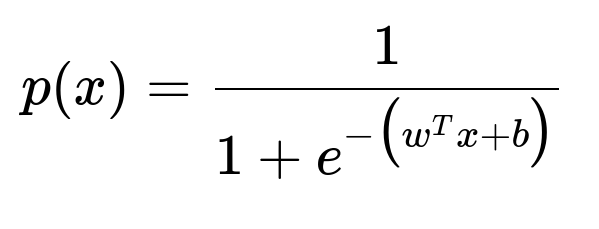
Here, w is the weight vector, x is the input feature vector, and b is the bias term. If one of the components in x is off by a factor of 100 (due to missing a decimal point), w^T x will become abnormally large or small, thus heavily distorting the value of p(x). This is why the model would no longer be valid: the distribution and scale of the data are no longer consistent with the original training set assumptions.
To address this, the usual approach is to correct the erroneous data by returning it to an appropriate scale. This involves identifying which data points have had their decimal removed and then adjusting them back to a normalized value. It often requires external knowledge of the data source (for example, you might discover that if the recorded value is unreasonably large compared to what was expected, you adjust it down by a factor of 100 or 1000 as needed). Once the fixes are applied, you typically retrain the model on the corrected data. In some cases, you might remove the corrupted records if you cannot ascertain the true values. The key idea is that your training data and inference data must have consistent scaling for the model to remain valid.
Potential Follow-Up Questions
How can you detect or prevent silent data corruption?
Data integrity checks are essential. One approach is to set validation rules or reasonableness checks on feature values, such as ensuring no observations exceed plausible thresholds. If a value is far outside the reasonable range, you can either flag or transform it. Automated sanity checks, anomaly detection techniques, and better data-collection practices can reduce the likelihood of these silent errors creeping into your modeling pipeline.
If you notice suspicious predictions during inference, how do you troubleshoot?
One strategy is to compare the distribution of new incoming data against the distribution of your training data. If you see that certain features in the new data exhibit drastically different ranges or statistical patterns, it suggests there may be data-quality issues. Visualizing histograms or box plots for these features helps expose whether decimals are being dropped or other errors are occurring. You can also run test predictions on a sample of known-correct inputs to verify the model’s calibration.
Is scaling the data (for example, using standardization) enough to fix the problem?
Standardization or normalization can help mitigate variation among different features, but it will not correct data that has been fundamentally corrupted by missing decimal points. If you standardize a feature set that includes values wrongly magnified by 100 or 1000, those points will still be outliers that skew the mean and standard deviation used in scaling. The correct step is to fix or remove the incorrect observations before or alongside any standardization.
Could a robust model like a tree-based method handle this type of corruption better?
Methods like random forests or gradient boosting can sometimes be more robust to outliers than logistic regression because they split features at certain threshold values rather than relying solely on linear transformations. However, severe corruption (like moving from 100 to 10000) can still degrade performance substantially, especially if the model encounters many erroneously large or small values. Ultimately, even if a model can be more tolerant, the best solution is still to correct the data.
How might you implement a quick fix in code if you discovered that only some values were multiplied by 100?
You could locate abnormally large records in your dataset, perhaps by an if condition such as if value > 999, then fix it by dividing by 100. You would need domain knowledge to decide exactly how to correct each erroneous value.
import pandas as pd

# Suppose 'df' is your dataframe and 'feature' is the problematic column
# Quick approach if you suspect values > 999 are off by exactly a factor of 100

df.loc[df['feature'] > 999, 'feature'] = df.loc[df['feature'] > 999, 'feature'] / 100.0

# Then retrain your logistic regression
from sklearn.linear_model import LogisticRegression

X = df.drop('target', axis=1)
y = df['target']

model = LogisticRegression()
model.fit(X, y)
By correcting obviously inflated values, you can often recover a cleaner distribution. However, a more robust solution would involve confirming exactly which records were corrupted, using domain knowledge or additional meta-data.
Below are additional follow-up questions
What if the corrupted decimal points vary by different factors (some off by 100, others by 1000)? How do you handle such inconsistent errors?
One of the main challenges arises when there is no single universal factor by which the data is off. You may have observations that should be 100 but appear as 10000 (a factor of 100 shift), while other instances should be 200 but appear as 200000 (a factor of 1000 shift). In such scenarios, you cannot simply apply a uniform rule like “divide by 100” to all outliers.
The best approach is often to perform a deeper data audit. This involves looking at the natural distribution of the feature you suspect is corrupted, possibly grouping or clustering data points according to their magnitude. If your domain expertise suggests that realistic values for this feature typically stay under 200, then any values significantly exceeding that threshold are potential candidates for corruption. You might then discover patterns that can help you differentiate between the different scaling errors (for instance, points in the tens of thousands might be off by 100, while points in the hundreds of thousands might be off by 1000).
You can also rely on auxiliary information from other features. For example, if you know from domain knowledge that the ratio of two features should never exceed a certain amount, you can look for rows violating that ratio to isolate the corruption. Regardless of the detection strategy, once you have identified the factor by which the values are off, you systematically correct them or remove them if the original factor cannot be confidently determined.
The key pitfall is assuming a one-size-fits-all fix. Inconsistent decimal shifts require more investigative work, including consulting business rules, subject-matter experts, or external logs that might give clues about the correct scaling factor. Without this, you might introduce further errors by applying incorrect corrections to your data.
How do you find the root cause of the decimal corruption in a real system, and why is this important?
Finding the root cause is crucial because merely cleaning up your training data doesn’t guarantee that future data will not have the same issue. In a production environment, if the data pipeline is still flawed, these errors can silently reappear, degrade model performance, and even lead to poor business decisions.
You typically start by tracing your data pipeline. That involves: Investigating data-collection scripts or web forms used to gather the values. Inspecting any intermediate transformations that might have inadvertently dropped decimal points, such as CSV parsing issues, type casting, or rounding errors in an upstream process.
Additionally, logs or system error reports can reveal if there were known system updates or misconfigurations around the time corruption started. Once identified, fix the pipeline at the source. This may involve updating code to ensure numeric precision is preserved, adding checks that enforce a particular format, or adopting robust data validation frameworks that raise alerts when suspicious values appear.
The subtle real-world issue is that these errors can sometimes show up only intermittently. If you’re not consistently monitoring your data distribution or logs, the corruption might remain undetected for a long time. Therefore, establishing a monitoring mechanism with alert thresholds based on typical value ranges is essential for catching such problems early.
In what situations would you consider leaving the corrupted data as is and rely on robust modeling or transformations?
Although the ideal solution is always to fix corrupted data at its source, there may be urgent scenarios where you have little time to fully correct the dataset. For example, consider a time-critical application where you cannot afford downtime for thorough investigation and repair.
You might then try employing robust methods that can handle extreme outliers. Tree-based ensemble methods (like Random Forests or Gradient Boosted Trees) are less sensitive to large magnitude changes in a feature since they rely on threshold-based splits. Additionally, transformations such as winsorizing (where extreme values are clipped to a certain percentile range) or applying a logarithmic transform can sometimes help reduce the impact of large corrupted values without precisely identifying and fixing each one.
However, even robust methods are not guaranteed to handle extreme, systematic shifts correctly. You risk losing a significant portion of your model’s fidelity if the corruption is pervasive. The real-world pitfall is that you might appear to get acceptable performance metrics during quick validation, but future predictions could be unreliable if the corruption pattern changes again or if new correct data arrives without the shift.
Could regularization in logistic regression mitigate the problem of extreme values?
Regularization techniques (like L2 or L1) help control the magnitude of coefficients in logistic regression to reduce overfitting. However, they do not inherently solve the problem of severely distorted input data. If a feature includes values that are off by a factor of 100 or 1000, these points still have an outsize influence on the loss function during training.
Even if the coefficients are small, a handful of extremely large feature values can dominate the product w^T x. As a result, the model’s predictions can swing unpredictably. While regularization might limit how massive the learned weights can become, the fundamental mismatch between the correct and corrupted data scales remains. In other words, regularization can partially reduce the damage but does not fundamentally correct the source of the error.
An edge case is if the corruption is relatively minor or if the feature is not heavily weighted by the model in the first place. Then regularization could help the model ignore that feature to some degree. Yet, if the feature is crucial to the prediction task, the best practice is still to restore the data to its correct scale.
What if you suspect only a portion of the dataset has decimal corruption, but you cannot confirm exactly which rows are erroneous?
Sometimes the corruption might be sparse or partial, and you lack a reliable indicator for which rows are incorrect. In this situation, you can explore anomaly detection methods to flag suspicious observations. For instance, isolation forests or robust covariance methods can help identify points whose magnitude or combination of features looks unusual compared to the rest of the dataset.
Once you isolate these suspicious samples, you can: Attempt to verify them against external data sources or logs. Decide on a systematic approach to either fix or remove them if no reliable fix is found.
The risk is discarding genuinely valid (but rare) points. This can happen if an event truly produced large feature values that are not corrupt. Domain knowledge is critical here to avoid discarding meaningful edge cases. You may also consider partial solutions like weighting less trusted data points lower in the training process or using semi-supervised anomaly detection to refine your approach.
How can you deal with real-time streaming data if decimal corruption is discovered mid-production?
When data arrives in a streaming fashion, you want to intercept corruption as early as possible to avoid polluting downstream systems and models. A recommended practice is to implement a real-time validation layer where each incoming data record is checked against a set of rules. If a feature’s value violates an expected range or pattern, the record is quarantined for further inspection. You might do a quick fix if the corruption factor is known, such as dividing by 100 or 1000 for values that clearly exceed normal bounds.
Meanwhile, you would alert the engineering or data team to investigate and permanently rectify the source of corruption. Throughout this period, you might keep a fallback model trained on the last known clean data, so that your main pipeline can continue operating with minimal downtime.
A subtle complication is that real-time constraints may not always allow for complex anomaly detection. You must balance computational overhead with the urgency of correct data processing. This is especially important in high-throughput systems where every millisecond matters. In such high-demand setups, you’d likely rely on simpler bounding rules or consistency checks rather than more computationally heavy algorithms.
What role can domain knowledge play in designing a more error-resistant feature?
Domain knowledge is often the strongest ally in preventing data corruption because it guides you in deciding not just what transformations to apply but also how to interpret raw inputs. For example, if you know the valid range of a measurement in your domain is between 0 and 500, you can outright reject or flag any value outside that range. You can also store data in standardized formats (such as integers representing cents instead of decimal floats) to reduce floating-point confusion.
In addition, domain expertise might inform you about relationships between features. If the variable in question is supposed to be correlated with another measurement, large deviations from that correlation could indicate data corruption. Armed with this knowledge, you can build cross-feature validation rules that automatically detect suspicious points.
The major pitfall is operating purely in a data-driven manner without leveraging domain insights. You may end up with partial fixes that seem statistically sound but miss the underlying reason for the corruption. Over time, a lack of domain alignment can allow subtle errors to resurface or go unnoticed.
What if retraining is costly or time-consuming, making it hard to re-fit the model after every data fix?
Frequent retraining can be expensive, especially with large datasets or complex models. If your pipeline or business environment does not permit immediate retraining after each fix, you might consider online learning or incremental learning techniques. These approaches update model parameters in smaller increments as new batches of cleaned data arrive, without completely restarting from scratch.
In logistic regression, for instance, there are stochastic gradient descent (SGD) variants that can continuously adjust the model coefficients. As soon as you correct a batch of data, you push it through the model again. This can be more efficient than a full retrain, as it leverages the prior parameters as a starting point. However, if the corruption significantly alters the data distribution, incremental updates might still struggle to converge correctly.
A potential edge case is that if your model has drifted too far due to long-term corrupted data, small incremental updates may not be sufficient to revert it. In that scenario, a full retraining becomes necessary once you have thoroughly cleansed the dataset.