ML Interview Q Series: If predictors are correlated in multiple linear regression, how does it affect outcomes and how to address it?

📚 Browse the full ML Interview series here.

Short Compact solution

If multiple predictors in a regression model are correlated, the estimated coefficients may fluctuate dramatically. In some cases, a predictor’s confidence interval might include zero, making it unclear whether an increase in that predictor’s value corresponds to a rise or fall in the response. As a result, important variables could appear insignificant if their effects are “split” across correlated features, which leads to misleading p-values and greater uncertainty over which predictors truly matter.

To manage this challenge, one approach is to remove redundant predictors once you confirm they are redundant. Alternatively, you can combine correlated predictors, for instance by generating interaction terms. It is also useful to investigate the source of the correlation to determine whether you have included effectively duplicated variables (like X and 2X) or whether certain underlying latent factors affect multiple predictors simultaneously. Centering the data, increasing the sample size, or applying regularization methods such as ridge regression are additional ways to reduce the instability in coefficient estimates.

Comprehensive Explanation

Multicollinearity arises when one or more predictors in a multiple linear regression are highly correlated. In a standard multiple linear regression setting, each coefficient is interpreted as the effect of that predictor on the response while other predictors are held constant. When two or more predictors share a strong correlation, holding them “constant” becomes practically impossible, and the model struggles to precisely separate their individual influences.

Coefficient Instability: When highly correlated variables exist, the matrix used to solve for coefficients can be close to singular, meaning it is nearly impossible to invert with precision. In ordinary least squares regression, the coefficient estimates are often found by a formula that, in simplified matrix form, looks like:

Misleading Significance: A high degree of correlation among predictors tends to inflate the variance of the estimated coefficients, leading to wide confidence intervals. Even genuinely important predictors can end up with large standard errors, making them appear insignificant in terms of statistical tests (e.g., large p-values). This uncertainty also makes it difficult to know which variable is actually driving the model.

Potential Remedies: Removing or combining correlated variables is one straightforward solution. If two variables are simply duplicates or linear transformations (such as X and 2X), one of them can be safely removed. In other cases, correlated variables may be combined via domain knowledge or by engineering new features (for example, an interaction or sum of the correlated predictors). Techniques such as ridge regression introduce a penalty on the size of coefficients, which helps keep them stable even if there is collinearity. Another approach is centering the data so that all features have mean zero, which can sometimes reduce correlation especially when interaction terms are introduced. Increasing the sample size can also help by providing more information for distinguishing each predictor’s effect.

If the Correlation Among Predictors Is Small, Is It Still a Problem?

Even when correlations between predictors are moderate rather than extreme, you may still encounter inflated variances in the coefficient estimates. This can lead to less reliable inferences but not necessarily to the same extent as severe collinearity. In general, minor correlations do not cause as much concern, but it is good practice to check for any relationships among the features and monitor whether they degrade model interpretability or significance in an unacceptable way.

How Can We Quantify or Detect Collinearity in Practice?

It is common to examine pairwise correlation coefficients or a correlation matrix to look for obvious relationships among predictors. Beyond pairwise correlation, the Variance Inflation Factor (VIF) is another tool: it measures how much the variance of a regression coefficient is “inflated” because of collinearity. If the VIF for a predictor is extremely high (some practitioners use thresholds like 5 or 10), it suggests that the associated coefficient is no longer reliable due to strong linear relationships with other variables.

How Do We Interpret Coefficients When There Is Correlation Among Predictors?

Coefficients in a multiple regression model are partial regression coefficients. Each coefficient represents the rate of change in the response variable while holding all other predictors constant. When predictors are correlated, holding one predictor constant while manipulating another is somewhat artificial because they move together in the real data. This does not invalidate the model, but it makes the interpretation more nuanced. It becomes more valuable to think in terms of the joint effect of a set of correlated variables.

How Might Principal Component Regression or Partial Least Squares Help?

Principal Component Regression (PCR) and Partial Least Squares (PLS) are dimension-reduction techniques. Instead of regressing the response on highly correlated predictors directly, these methods transform the predictor space into new variables (principal components or latent vectors) that are linear combinations of the original features. By using fewer components (which capture the majority of the variance in the predictors), you bypass the instability that arises from collinearity. However, the trade-off is that interpretation in the original predictor space may become more difficult, since you are interpreting combinations of variables rather than individual variables themselves.

Would Lasso or Ridge Regression Be Better for Handling Multicollinearity?

Both ridge and lasso regression apply regularization to the coefficients and can reduce the impact of collinearity. Ridge regression shrinks coefficients toward zero in a way that distributes shrinkage across correlated predictors. It does not typically drive any single predictor’s coefficient exactly to zero, but it stabilizes the estimates and handles multicollinearity very well. Lasso (L1 penalty) can actually set some coefficient estimates to zero, effectively performing feature selection. If there is a group of correlated predictors, lasso tends to pick one or a few from that group to keep in the model and zeroes out the rest. This can be a practical way of tackling redundancy in correlated predictors, but it may be somewhat unstable when many variables have strong correlations and similar explanatory power.

Is It Always Best to Remove Correlated Variables, or Are There Times We Might Keep Them?

There are situations where correlated variables carry distinct meaning and domain-specific importance. For instance, two highly correlated economic indicators might still be conceptually different and each one could be independently important for policy interpretation. Removing them might lose valuable nuance. In other cases, the objective of the model might be predictive accuracy rather than interpretability. Keeping correlated predictors could be beneficial if they collectively improve predictions (especially under regularization methods). The decision hinges on balancing interpretability with predictive goals and domain knowledge.

When the ultimate goal is interpretability, removing or combining correlated predictors (or using an alternative modeling strategy) can often be preferable. If the goal is purely predictive performance, techniques like ridge regression might allow you to keep all variables while maintaining stable predictions.

Practical Code Example in Python

Below is a brief illustration in Python of how one might examine and address multicollinearity in a dataset:

import pandas as pd
import numpy as np
from sklearn.linear_model import LinearRegression, Ridge
from statsmodels.stats.outliers_influence import variance_inflation_factor

# Example dataset with potential collinearity
np.random.seed(0)
N = 100
X1 = np.random.randn(N)
X2 = 2 * X1 + np.random.randn(N) * 0.01  # Correlated with X1
X3 = np.random.randn(N)
y = 3 * X1 + 1.5 * X3 + np.random.randn(N)

# Put into a DataFrame
df = pd.DataFrame({'X1': X1, 'X2': X2, 'X3': X3, 'y': y})

# Examine correlation matrix
print(df[['X1','X2','X3']].corr())

# Compute VIF for each feature
X_mat = df[['X1','X2','X3']]
vif_data = []
for i in range(X_mat.shape[1]):
    vif = variance_inflation_factor(X_mat.values, i)
    vif_data.append((X_mat.columns[i], vif))
print(vif_data)

# Ordinary Linear Regression
lr = LinearRegression()
lr.fit(X_mat, df['y'])
print("Linear Regression Coefficients:", lr.coef_)

# Ridge Regression to handle collinearity
ridge = Ridge(alpha=1.0)
ridge.fit(X_mat, df['y'])
print("Ridge Regression Coefficients:", ridge.coef_)

In this example, X2 is highly correlated with X1. The correlation matrix and VIF values would confirm the collinearity. The Ridge regression’s coefficients would typically be more stable (smaller absolute values and less variance) compared to standard linear regression, indicating how regularization mitigates the impact of correlation.

By examining the correlation matrix, calculating VIF, or simply observing unexpected coefficient signs or large standard errors, we can diagnose collinearity and then decide whether to remove, combine, or apply regularization to the predictors.

Below are additional follow-up questions

What if correlation among predictors reflects something meaningful and not just redundancy?

When predictors are correlated in a way that reflects meaningful relationships in the domain, removing them simply to reduce collinearity may discard useful information. For instance, economic indicators often move in tandem because of an underlying macroeconomic condition—one indicator might capture consumer confidence, while another captures employment rate, and they naturally move together. Edge cases/pitfalls:

• If you remove or combine these correlated predictors without a deep understanding of the domain, you might obscure genuinely different signals.

• An overly simplistic approach might collapse multiple indicators into a single feature that then loses distinct interpretive power. This is problematic when stakeholders rely on the separate variables to make specific policy decisions or operational changes. How to handle:

• Check domain literature to confirm whether those variables measure separate constructs.

• Consider partial correlation analysis or domain-informed transformations to better isolate each predictor’s unique effect.

• If interpretability is key, you may keep both but use techniques like ridge regression to reduce coefficient variance.

How do you deal with correlated variables in contexts outside of linear regression, such as tree-based methods?

Tree-based ensemble methods like random forests, gradient boosting, or decision trees are often far less sensitive to collinearity. This is because trees partition the feature space based on threshold splits, and correlated features do not destabilize the splitting process as much. However, correlated features can still impact variable importance measures. Edge cases/pitfalls:

• If two features are highly correlated, the tree might pick one of them more often for splits, making the other one appear less important in standard importance metrics (e.g., Gini importance), even though both are essentially carrying similar predictive information.

• In extreme cases where two features are near duplicates (X and X+0.0001 noise), many tree splits might get “wasted” on essentially the same information, slightly increasing computational cost. How to handle:

• You might remove or combine near-duplicate features for efficiency.

• You could use permutation-based importance (testing the impact on the model’s error rate) rather than standard Gini importance to get a fairer sense of each variable’s true contribution.

• If interpretability is critical, you still need to decide which of the highly correlated features to keep in your final model or provide them together but highlight that they carry similar information.

Does multicollinearity have a role in time series analysis or panel data?

In time series or panel data, certain predictors naturally move together over time (e.g., temperature and electricity usage). Moreover, lagged versions of the same variable can exhibit high correlation. Edge cases/pitfalls:

• If you use differencing or seasonality adjustments, sometimes you reduce the correlation among the original variables but may introduce new correlations across time-lagged terms.

• In panel data where each entity (e.g., each individual, store location, or region) is tracked across time, you may have correlated variables that differ primarily across entities. Failing to account for entity-specific effects can inflate the correlation structure in the regression errors. How to handle:

• Consider using specialized methods (e.g., Vector Autoregression, fixed-effects models, random-effects models) that explicitly model the temporal or cross-sectional dependence.

• Check correlation structures not just in the raw data but also in residuals to ensure you have properly accounted for repeated measures or time lags.

Can correlated predictors cause issues in logistic regression or other generalized linear models (GLMs)?

Logistic regression and other GLMs still rely on maximum likelihood estimation, which requires stable coefficient estimates. Correlated predictors can lead to large standard errors and unstable parameter estimates, much like in linear regression. Edge cases/pitfalls:

• Perfect or near-perfect collinearity in logistic regression may cause complete separation, where the model cannot converge because the likelihood goes to infinity (or the gradient fails to converge).

• You might see extremely large magnitude coefficients or parameter estimates that fail to stabilize during optimization. How to handle:

• Use regularization (e.g., elastic net or ridge penalty) to stabilize the estimates.

• Investigate variance inflation for logistic regression or use correlation checks to see if a subset of predictors can be removed.

• In cases of complete separation, methods like Firth’s bias-reduced logistic regression can provide finite and stable coefficient estimates.

Does scaling or normalizing correlated features help reduce collinearity?

Scaling (e.g., standardizing to have zero mean and unit variance) usually does not eliminate correlation since it is a linear transformation applied feature by feature. The correlation structure typically remains the same. However, certain transformations can reduce correlation if they alter the relationship’s shape. Edge cases/pitfalls:

• A log transform could reduce correlation if the relationship between two variables is multiplicative rather than additive, but applying it blindly can distort interpretability or lose valid zero or negative values.

• Polynomial expansions or piecewise transforms can inadvertently create new collinearities if all polynomial terms strongly correlate. How to handle:

• Before applying any transformation, explore how variables relate to each other (e.g., do they appear to have a multiplicative pattern?).

• After transformations, re-check correlation and interpretability.

• Consider domain-based transformations known to linearize relationships rather than ad hoc transformations.

In practical terms, how do we decide a threshold for “too high” correlation?

A common heuristic is that a pairwise correlation coefficient above 0.8 or 0.9 might cause concern. However, the significance of correlation depends on the problem, the sample size, and the number of predictors. Edge cases/pitfalls:

• Relying solely on a single cutoff can lead to ignoring moderate but still problematic correlations, especially in small sample scenarios.

• Very large sample sizes might sustain a higher correlation threshold without inflating variance too severely. Conversely, smaller samples are more vulnerable even at moderate correlation levels. How to handle:

• Use domain knowledge to set context-specific thresholds. For example, if it is known that two features represent nearly the same measurement, even a correlation of 0.7 could be grounds for concern.

• Complement correlation analysis with VIF to capture multi-way dependencies.

Can we detect multicollinearity visually?

Yes, partial regression plots (also called added-variable plots) and correlation heatmaps are two common visualization approaches. Partial regression plots show how a specific predictor relates to the response after adjusting for other predictors. Edge cases/pitfalls:

• Visual inspection can be subjective; you might misinterpret the scale or pattern in a partial regression plot, especially when the data set is large.

• Correlation heatmaps only show pairwise correlation, so they can overlook complex multi-way collinearities that involve multiple features simultaneously. How to handle:

• Combine visualization with numeric diagnostics (like VIF). If partial plots appear nearly flat or extremely noisy, it may hint that a predictor’s effect is confounded by other correlated predictors.

• For large data sets, consider random down-sampling for visualization so your plots remain interpretable and do not become overcluttered.

How does multicollinearity affect confidence intervals and prediction intervals differently?

With high correlation, the coefficient confidence intervals inflate, reflecting uncertainty in the parameter estimates. However, the overall model might still predict the target variable reasonably well. Edge cases/pitfalls:

• You could have decent prediction accuracy but lose clarity about which variables are most influential. This is a problem when the primary goal is inference or explanation rather than pure prediction.

• For prediction intervals (the uncertainty in actual predictions for new observations), if the correlation structure in new data matches the training data, the aggregated effect from correlated predictors might remain stable, so your predictions remain accurate. But if that correlation structure changes (covariate shift), your predictions might degrade rapidly. How to handle:

• Check both coefficient confidence intervals and out-of-sample prediction error.

• If interpretability is key, invest more time in diagnosing which coefficients cannot be reliably estimated. If pure prediction is the goal, a method robust to collinearity (like ridge or ensembles) might suffice, and wide coefficient intervals might be acceptable.

What if correlation in the data shifts over time or across subpopulations?

In many real-world scenarios, the relationship between features evolves. Features might be correlated under one set of conditions but become less correlated (or even inversely correlated) under another set of conditions (e.g., during a market shift). Edge cases/pitfalls:

• A model trained on historical data might assume certain correlations that no longer hold. Coefficients might become unreliable, leading to poor predictions or misguided policy decisions in new conditions.

• You may see abrupt changes in the sign or magnitude of your variable relationships if a major event alters the underlying data-generating process. How to handle:

• Continuously monitor model performance and correlation structure over time.

• Retrain or update the model if you detect significant drifts in feature correlations.

• Consider online learning or time-adaptive strategies that adjust coefficients as new data arrives.

Can rank deficiency occur, and what does it mean in practice?

Rank deficiency occurs when your design matrix X does not have full column rank—i.e., one or more columns are linear combinations of others. This can happen if you include dummy variables that sum to a constant or if you have an exact linear relationship among numeric features (like X2 = 2 * X1). Edge cases/pitfalls:

• Your linear algebra solver may fail or produce infinite solutions for the coefficient estimates. Some software handles it by dropping one of the redundant columns automatically, but you may be unaware which one was dropped.

• With complicated data pipelines, such redundancies might inadvertently creep in (for example, a feature derived from others or one-hot-encoded categories incorrectly specified). How to handle:

• Before fitting the model, check for perfectly collinear or redundant features.

• Make sure any categorical encoding is performed in a way that avoids the dummy variable trap (e.g., for one-hot encoding, drop one base category).

How do we manage correlated predictors in situations where the model will be used for causal inference?

Causal inference typically relies on carefully ensuring that the included variables are confounders or mediators as per a causal diagram, rather than simply predictive features. Correlations among predictors can confound effect estimates if some of those variables are mediators or colliders. Edge cases/pitfalls:

• Standard regression assumptions do not necessarily hold in the presence of post-treatment variables or colliders. High correlation might result from a causal pathway (e.g., X influences Z, and both X and Z predict Y).

• Controlling for a collider can actually introduce bias, so removing or combining features solely based on correlation might disrupt a well-structured causal model. How to handle:

• Use a causal framework (e.g., directed acyclic graphs, potential outcomes) to determine which variables you should include or exclude.

• If correlation arises because of a mediator, reflect on whether you actually want to estimate the direct effect (exclude mediator) or total effect (include mediator).

What if we suspect non-linear relationships among correlated predictors?

Collinearity diagnoses (like VIF and correlation measures) are primarily for linear relationships. Non-linear relationships can be missed if variables are only correlated under certain ranges or have different slopes at different values. Edge cases/pitfalls:

• You may incorrectly assume you have “fixed” collinearity at the linear level, only to discover more subtle relationships that remain unaddressed. How to handle:

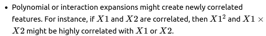
• Apply correlation checks not only to the raw features but also to any polynomial or interaction terms you generate.

• Use advanced diagnostic tools (e.g., generalized additive models, partial dependence plots) to see if non-linearity is introducing hidden collinearity.

Could correlated predictors be a sign of data leakage?

Data leakage can occur if one predictor implicitly encodes the response or includes future information. If your “predictors” are highly correlated because one of them is effectively the “answer,” you may see artificially strong predictive performance. Edge cases/pitfalls:

• In time-sensitive scenarios, a variable measured in the future might correlate strongly with a predictor from the past, thus leaking future data into training. This leads to inflated estimates of model accuracy but fails in real-world deployment.

• If a derived feature incorrectly includes some portion of the target variable (perhaps via a mislabeled data pipeline step), correlation with the rest of the features might skyrocket. How to handle:

• Double-check the data collection timeline to ensure each predictor is measured before the target outcome.

• Evaluate the real-world feasibility of each predictor. If it is suspiciously perfect or near-perfect in correlation with the outcome, investigate whether it indirectly encodes the outcome.

Is dimensionality reduction always necessary when dealing with many correlated features?

Dimensionality reduction like PCA is often a quick fix to reduce large sets of correlated features. However, it can obscure the interpretability of individual variables. If your aim is prediction and you do not need the original feature semantics, PCA might work well. Edge cases/pitfalls:

• Blindly applying PCA could merge features that should remain separate due to domain requirements (e.g., merging “humidity” and “temperature” into a single principal component might be unhelpful for certain climate interventions).

• If your data are extremely high-dimensional (e.g., thousands of correlated genetic markers), PCA or other methods might be essential to avoid overfitting, but ensure you keep track of how many components to retain. How to handle:

• Use domain expertise to identify which variables can be combined meaningfully.

• Compare performance and interpretability trade-offs between raw correlated features vs. transformed principal components.

• If interpretability is critical, partial least squares or supervised dimensionality reduction methods might provide more interpretable solutions than standard PCA.