
ML Interview Q Series: Imagine a default risk model where its recall is high but its precision is relatively low. What implications could this have for a mortgage provider?

📚 Browse the full ML Interview series here.
Comprehensive Explanation
High recall but low precision means that the model correctly identifies most of the actual defaulters but also flags a substantial number of non-defaulters as potential risks. To clarify, recall and precision for a binary classification task can be expressed by the following core formulae:

Right below this formula, in text-based math, True Positives (TP) refers to loans correctly identified as default risks, while False Positives (FP) refers to loans that the model incorrectly labeled as default risks even though they would not actually default.

Below this, True Positives (TP) again are actual defaulting loans that the model flagged correctly, and False Negatives (FN) are those loans that the model missed, labeling them as safe even though they end up defaulting.
A high recall means almost all potential defaulters are being caught. A low precision, however, means the model is raising too many false alarms on borrowers who likely would not default. When translated to a mortgage bank’s day-to-day operations, this can lead to the following real-world implications in very practical terms:
The bank might approve fewer loans than it ideally could, because it is overly cautious with many borderline borrowers. The cost of investigating or rejecting these false-positive cases goes up, since the bank might have to allocate additional resources (such as more rigorous manual underwriting steps, increased staffing to review flagged applications, or additional compliance checks). Despite correctly catching most truly risky borrowers, the bank’s profitability might be impacted by turning away potentially good customers or imposing higher interest rates on them. This can diminish customer satisfaction and reduce the bank’s competitive edge if other institutions have more accurate targeting.
Additionally, from a strategic standpoint, a low-precision but high-recall model might instill a sense of security against defaults (because it catches most actual defaulters), but it also imposes an implicit cost or lost opportunity on customers who do not truly pose a risk.
A balanced approach often requires calibrating the decision threshold for the classifier to strike a suitable tradeoff. That way, the bank can choose an operating point that is mindful of both the cost of false positives (potential revenue loss and negative customer experience) and the cost of false negatives (actual defaults leading to financial losses and risk of regulatory scrutiny).
How Could We Measure and Balance Precision and Recall More Effectively?
In practice, data scientists often analyze the Precision-Recall curve or the ROC curve for the classification model. By adjusting the probability threshold used to decide whether a loan application is labeled “risky,” the bank can attempt to find a more effective operating region. The final threshold is typically chosen based on specific cost-benefit or risk tolerance scenarios: for example, the cost of missing a true defaulter might be far greater than the cost of false-positive investigations, or vice versa.
Using cross-validation on historical loan data with known outcomes can help the bank test a range of thresholds and observe the tradeoffs in terms of net profit or net loss. This is combined with domain knowledge: if the bank is in a period of economic uncertainty, it might prefer a more conservative approach, emphasizing high recall while accepting lower precision.
Follow-up Questions
Could you provide more insight into calculating precision and recall for a default risk model?
Precision and recall are derived from confusion matrix components (true positives, false positives, true negatives, false negatives). In a default risk context, a “positive” is a loan that is predicted to default. The model is typically run over a set of historical loans with known outcomes. For each loan, the model produces a predicted label (default or not). By aggregating predictions, you determine:
True Positives: Borrowers who truly defaulted and were predicted to default.
False Positives: Borrowers who did not default but were predicted to default.
True Negatives: Borrowers who did not default and were predicted not to default.
False Negatives: Borrowers who actually defaulted but were predicted not to default.
In code, you might generate predictions on a validation dataset and then compute:
from sklearn.metrics import precision_score, recall_score

precision = precision_score(true_labels, predicted_labels)
recall = recall_score(true_labels, predicted_labels)

print("Precision:", precision)
print("Recall:", recall)
How would we choose an appropriate threshold to balance these metrics?
The default threshold is often 0.5 for probabilities from a classifier, but you can adjust this threshold to trade off between precision and recall. A lower threshold increases recall (more loans labeled as potential defaults) but typically lowers precision. A higher threshold may improve precision (fewer false positives) at the risk of missing actual defaulters.
To find a suitable threshold:
Generate probabilities for the default class from the model.
Evaluate a range of thresholds (e.g., from 0.0 to 1.0 in small increments).
Compute precision, recall, or the F1 score for each threshold.
Plot the Precision-Recall curve or ROC curve and identify a threshold that aligns with the business’s risk and cost preferences. This might involve analyzing cost of false alarms vs. cost of actual defaults.
What is the relationship to Type I and Type II errors in this scenario?
Type I error (false positive) is labeling a non-defaulter as a defaulter. Type II error (false negative) is failing to identify a defaulter. High recall but low precision means we have fewer Type II errors (we catch most defaulters) but more Type I errors (we unnecessarily label many good customers as risky). Whether this is acceptable depends on the financial and reputational cost of turning away potentially good borrowers compared to the cost of taking on risky borrowers who might default.
How do real-world factors and cost structures influence the model’s acceptable tradeoff?
Real-world mortgage lending involves multiple costs: the cost of carrying a default (e.g., foreclosure, legal fees, loss of principal) and the cost of false positives (lost revenue, opportunity cost, and customer dissatisfaction). These factors can be translated into a cost matrix. For instance, if the cost of default is extremely high compared to the cost of false positives, a business might tolerate a lower precision and maintain a high recall. Conversely, if capturing potentially profitable customers is critical and the cost of default is partially mitigated by collateral or insurance, the business may aim for a more balanced approach or higher precision.
How might the bank mitigate the impact of high false-positive rates?
A multi-stage or multi-level model can be set up: the initial stage (model) flags a pool of possibly risky borrowers with relatively high recall (ensuring few missed defaulters). A second stage involves a deeper manual or semi-automated investigation of only those flagged applicants, using additional data sources or more sophisticated underwriting. This approach can reduce unnecessary rejection of creditworthy applicants while still catching most genuine defaulters.
The bank might also segment customers by risk profile or by loan product type. That is, a model could route borderline applicants into different underwriting tracks. This approach is sometimes combined with cost-sensitive learning or additional verification steps (e.g., verifying employment, prior payment history, additional collateral requests) based on the predicted risk category.
By implementing such layered strategies, the business can avoid blanket rejections for all flagged borrowers and thus mitigate the financial and reputational downsides of a low-precision model.
Below are additional follow-up questions
How might an economic downturn affect the balance between precision and recall?
In a recession or broader economic slowdown, default rates tend to rise, and the predictive patterns in training data might shift. A model built on historical data from more stable times may struggle to maintain its original tradeoff between catching defaulters (high recall) and avoiding unnecessary denials (precision). As more borrowers experience financial distress, typical feature distributions like income stability or loan-to-value ratios might not reflect reality anymore. This drift can lead to:
Increased false negatives if the model underestimates the severity of new economic conditions.
A potential need for re-calibration or retraining on more recent data that better captures evolving risk profiles.
Greater emphasis on recall to ensure defaulters are not missed, because the cost of a default may be higher during economic turmoil. This, however, might exacerbate lower precision, especially if the model now overcompensates for risks in ambiguous cases.
Effectively, the bank might adopt stricter acceptance criteria, but it should also regularly monitor model performance metrics and revise thresholds as the economic landscape evolves.
Could changes in borrower risk profiles over time lead to concept drift, and how can it be addressed?
Concept drift occurs when the relationship between input features and target outcomes changes over time. For a default risk model, macroeconomic factors (interest rate changes, employment rates, etc.) or shifts in consumer behavior (e.g., more gig-economy workers) can alter underlying risk patterns. Concept drift can degrade the model’s performance if it is not updated to reflect new realities. Strategies include:
Periodic Retraining: Regularly retraining the model on the most recent data to capture evolving borrower characteristics.
Online Learning: Continuously updating model parameters as new loan performance data becomes available.
Ensemble Approaches: Using multiple models trained on different time windows to capture a range of economic conditions, then combining their predictions.
Monitoring Mechanisms: Setting up thresholds or triggers that alert when performance metrics—like precision, recall, or overall accuracy—drop below acceptable levels, prompting a more thorough review.
Are definitions of “default” standardized across different regulatory environments, and how does that impact precision vs. recall?
Different jurisdictions and regulatory bodies can define “default” in slightly varying ways—some might consider a loan “in default” after one missed payment, others might require three consecutive missed payments or a specific percentage of principal outstanding. This affects the model’s labeling of positive cases. If a bank operates across regions with different standards:
The ground truth for training can vary and complicate a single global model approach, since a “default” in one region may not be considered as such in another.
The bank must carefully align its positive class definition with local regulations to avoid compliance risk or misclassifying loans.
Precision and recall can shift drastically if the threshold for what counts as default is changed. Adopting region-specific models or applying region-specific post-processing rules on a unified model may be needed to ensure consistent performance metrics.
How might the strategy change if the bank employs risk-based pricing rather than a simple approve/reject decision?
When using risk-based pricing, the bank does not outright reject borderline applicants. Instead, it adjusts loan terms (interest rate, collateral requirements, etc.) based on predicted risk. In this scenario:
Low precision is less damaging since false positives (borrowers incorrectly labeled high-risk) might still be given a loan, albeit with a higher interest rate, protecting the bank to some extent.
High recall remains crucial, so the bank can identify truly risky borrowers and assign appropriate risk premiums.
The bank must carefully analyze whether the additional costs to customers might lead to increased credit attrition or unintended fairness issues (for example, unfairly high rates for certain groups if the model is biased).
Threshold tuning can focus on different outcomes, such as segmenting the risk into tiers (low, medium, high) rather than a strict binary decision.
What are approaches to incorporate cost-sensitive learning into the model to handle imbalanced outcomes?
Cost-sensitive learning treats different types of classification errors with specific penalties. In a default risk model, it is often more costly to miss a true defaulter (false negative) than to mistakenly flag a non-defaulter (false positive). One way to incorporate this into logistic regression is by weighting positive and negative classes differently. A generic weighted loss function can be represented as:
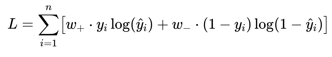
Here, w_{+} and w_{-} are the weights for positive (default) and negative (non-default) examples respectively, y_{i} is the actual outcome, and \hat{y}_{i} is the model’s predicted probability.
By assigning w_{+} > w_{-}, the model penalizes missed defaulters more heavily. This typically increases recall but may reduce precision.
Hyperparameter tuning of w_{+} and w_{-} can be guided by domain knowledge of the relative costs of false negatives vs. false positives, or by internal/external regulatory policies.
Modern frameworks (e.g., XGBoost, LightGBM) have built-in parameters (e.g., scale_pos_weight) for cost-sensitive training in imbalanced classification scenarios.
How can explainability methods help validate precision and recall tradeoffs with stakeholders?
In mortgage lending, regulators and internal stakeholders (e.g., risk management, compliance teams) must be convinced the model is not only accurate but also fair and explainable. If the model yields high recall at the expense of precision, many customers will be scrutinized or subjected to unfavorable terms. Explainable AI (XAI) techniques help in:
Uncovering which features drive the classification outcomes (e.g., income stability, past delinquency, debt-to-income ratio).
Identifying patterns that might suggest model bias or unintentional discrimination.
Communicating to decision-makers why certain loan applications are flagged as risky, possibly leading to better acceptance of a model with low precision but high recall in the short term.
Detecting inconsistencies or “unusual” feature interactions that might indicate a need for model refinement.
Can we combine multiple models to handle different segments of borrowers and improve overall precision and recall?
Segmentation is a practical solution if the mortgage portfolio spans distinct borrower groups. For instance, first-time buyers, self-employed individuals, or high-net-worth customers often exhibit very different risk profiles. A single global model can suffer from underfitting certain segments or producing too many false positives in others. A segmented approach might entail:
Building specialized models for each segment (e.g., a model for self-employed applicants where income variability is a key factor).
Using a global classifier first to route applications to a relevant specialized classifier, improving the precision-recall tradeoff in each subpopulation.
Ensuring each sub-model is regularly monitored for concept drift within its own domain.
Balancing complexity against the operational feasibility of maintaining and updating multiple models, as more specialized models require more robust infrastructure and staff expertise.
What challenges arise if the default label has a long lead time?
If default is only observed months or even years after the loan origination, then:
The feedback loop is significantly delayed, which may slow retraining or hamper the ability to detect new patterns.
Borrower conditions can change substantially during that time, making certain features at origination less predictive.
The model might need additional dynamic inputs (like interim payment behavior, changes in credit score, updated employment status) to maintain relevant precision and recall over the life of the loan.
Data engineering challenges can emerge, as the bank must track evolving borrower features over multiple time windows. A rolling or incremental approach might be required to keep the model updated.
In what ways might data quality issues affect the performance and reliability of precision vs. recall tradeoffs?
Data anomalies—such as incomplete employment history, under-reported income, or inconsistent credit bureau records—can introduce biases or inaccuracies:
Missing or noisy data can reduce precision if legitimate good borrowers are flagged due to insufficient information or spurious correlation.
Underreported defaults or slow updates on delinquency status can lead to inflated recall (because the model might treat incomplete negatives as true negatives).
Data validation, feature engineering best practices, and robust data pipelines (including automated checks for missing or inconsistent values) are essential to ensure that the precision-recall tradeoff reflects actual risk and not merely data artifacts.
Are there strategic scenarios where a business might intentionally accept a model with lower precision?
Yes, especially during times of high uncertainty—like new product launches or expansions into untested markets—some financial institutions prefer to prioritize capturing any possible signs of default risk (maximizing recall). This approach minimizes the chance of catastrophic losses if many new borrowers default at once, though it can hamper growth by turning away or scrutinizing potentially profitable segments. Over time, once the model has more data and a clearer understanding of the new market, the bank can refine the precision-recall balance toward improved customer acquisition while still managing risk.