ML Interview Q Series: Imagine you have built a new model to predict how long it will take for food deliveries to arrive. How can you verify that this updated model outperforms your existing one?

📚 Browse the full ML Interview series here.

Comprehensive Explanation

One of the most critical steps when introducing a new delivery time estimate model is to compare it systematically against the old model. We generally seek to determine whether the new model leads to smaller prediction errors, better alignment with actual delivery times, and improved performance under realistic business conditions.

Offline Evaluation Using Historical Data

A standard first approach involves comparing both models on a dataset of historical deliveries, each with known actual delivery times. You split these historical records into training and testing subsets or use a cross-validation approach. Your new model is trained on the training set, while the old model is already established. Then, both models produce predictions on the test set. You compare their errors using suitable metrics.

Selecting the Right Metrics

Delivery time predictions can be evaluated using regression metrics. Two of the most common are Mean Squared Error and Mean Absolute Error. These are typically used to measure how far the predicted values deviate from the actual values over all samples.

Mean Squared Error (MSE)

Use MSE if you want a metric that penalizes larger errors more heavily. This can be helpful when large deviations in predicted delivery times are especially undesirable. The central formula for MSE is often written as:

Where:

• n is the total number of data points in your test (or validation) set.

• y_i is the actual delivery time for the i_th data point.

• hat{y}_i is the predicted delivery time for the i_th data point.

• (hat{y}_i - y_i)^2 represents the squared error for that data point.

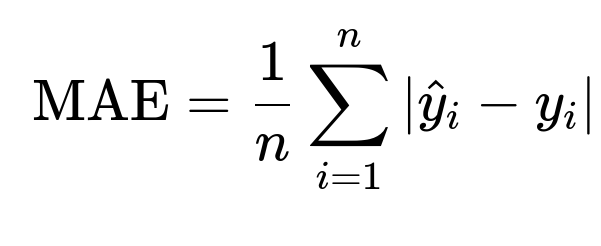
Mean Absolute Error (MAE)

If you want a metric that is more robust to outliers and directly measures average absolute deviation, you can use MAE. The core formula for MAE is:

Where:

• The notation remains consistent with MSE, but the absolute error is used instead of squared error.

Comparing Models Statistically

Even if the new model's average error is lower, you should assess whether the difference is statistically significant. Standard techniques, like a paired t-test on the error distributions, can help you confirm whether performance improvements are robust rather than due to random chance.

Online or Live Testing (A/B Testing)

Beyond offline evaluation, it is often essential to test the new model live. You can run an A/B test where some percentage of users see the old model’s predictions and others see the new model’s predictions. You then measure:

• Actual delivery times vs. predicted times.

• User satisfaction (e.g., complaints regarding delays or inaccurate estimates).

• Potential effects on order flow (whether users are discouraged if the predicted time is too high).

A/B testing provides real-world evidence that the new model maintains or improves the user experience and aligns well with actual outcomes.

Considerations Beyond Accuracy

Even if your new model appears to reduce error, you might also care about:

• Bias: Does the model consistently underestimate or overestimate delivery times?

• Distribution of errors: Are errors more concentrated or do they have heavy tails?

• Robustness: How does the model handle scenarios of peak hours, inclement weather, or unexpected traffic?

• Scalability: Does the new model have higher computational or memory demands that could impact production systems?

All these factors feed into whether the new model is genuinely "better" in a real operational sense.

Follow-up Questions

How would you handle outliers in the dataset, such as extremely long or short delivery times?

Outliers often arise due to special circumstances, like severe traffic, restaurant delays, or user cancellations that might misrepresent true delivery behavior. When measuring performance:

• You could cap or trim extreme values. For instance, remove the top 1% and bottom 1% of records to reduce noise.

• You could use more robust metrics like Median Absolute Deviation, which are less sensitive to extreme values.

• You might create separate models or special rules for unusual circumstances (e.g., bad-weather mode). This ensures that you do not distort overall performance by forcing the model to account for extremely rare cases under normal conditions.

What if your new model is more accurate on average but frequently underestimates actual times?

Underestimations can cause significant user dissatisfaction because customers might be more frustrated when deliveries arrive later than promised. In such a scenario:

• You could employ a cost function that penalizes underestimations more than overestimations. That might involve a weighted loss for negative errors.

• You can measure the direction of the errors using metrics like Mean Signed Error to see if the model systematically underestimates times.

• You might combine both average accuracy metrics (like MAE) with percentile-based metrics to assess whether the model is often too optimistic.

How do you ensure your tests are statistically sound, especially in an A/B test?

• Use confidence intervals and appropriate statistical tests (like a two-sample t-test) to check the significance of the performance difference between control (old model) and treatment (new model).

• Ensure a large enough sample size in the A/B test to detect meaningful differences with sufficient statistical power.

• Monitor p-values along with effect sizes, since practical significance matters as well as statistical significance.

Could you show a simple example in Python to compare the errors of two models?

import numpy as np
from sklearn.metrics import mean_squared_error, mean_absolute_error

# Suppose y_true is a NumPy array of actual delivery times
# y_pred_old is a NumPy array of predictions from the old model
# y_pred_new is a NumPy array of predictions from the new model

y_true = np.array([30, 45, 60, 35, 50])
y_pred_old = np.array([25, 50, 70, 40, 55])
y_pred_new = np.array([28, 46, 63, 33, 48])

mse_old = mean_squared_error(y_true, y_pred_old)
mse_new = mean_squared_error(y_true, y_pred_new)

mae_old = mean_absolute_error(y_true, y_pred_old)
mae_new = mean_absolute_error(y_true, y_pred_new)

print("Old Model MSE:", mse_old)
print("New Model MSE:", mse_new)
print("Old Model MAE:", mae_old)
print("New Model MAE:", mae_new)

You can run such an evaluation and compare metrics side by side. A lower MAE or MSE for the new model indicates it is more accurate in predicting delivery times, at least under these test conditions.

What would you do if your model’s overall accuracy improves, but certain regions or restaurants show worse performance?

• Segment the evaluation by different geographies, restaurant types, or times of day.

• Investigate whether these segments have unique behaviors that the new model is not capturing.

• Consider training specialized models (e.g., per-region models) or adding features specific to those segments.

By exploring per-segment performance, you ensure that improvements are genuinely widespread and not driven by a majority group at the cost of minority cases.

Below are additional follow-up questions

How would you design a cost function that imposes heavier penalties for late deliveries compared to early ones?

A direct way to tackle the asymmetry between overestimation and underestimation is to modify your loss function to penalize late deliveries more severely. One approach is to apply a weight factor that scales the loss term when actual delivery time is greater than the predicted time.

For a simplified weighted MSE concept, you could use:

Where:

• n is the total number of data points.

• y_i is the actual delivery time for data point i.

• hat{y}_i is the predicted delivery time for data point i.

• w_i is a weight factor that might be larger when hat{y}_i < y_i, causing underestimation.

One pitfall is deciding on w_i. If w_i is set too high for late deliveries, the model might over-correct and start giving overly conservative predictions, frustrating users who receive deliveries earlier than expected. Conversely, if w_i is too low, you do not solve the underestimation problem effectively. Tuning w_i involves carefully balancing real-world business constraints, user satisfaction data, and domain knowledge about how late vs. early deliveries affect the service.

How do you update predictions in real-time as traffic conditions or restaurant delays change?

Delivery environments can be dynamic. Predicting a static time at the moment the order is placed might quickly become inaccurate if traffic conditions worsen, the restaurant falls behind, or a driver is delayed.

You could:

• Continuously poll or receive events that represent changes in traffic, restaurant preparation stages, and driver availability.

• Recompute the delivery estimate using a model that can quickly retrain or adjust parameters in near real-time. If full retraining is expensive, you could use a simpler, lightweight model or incremental learning that adjusts based on the most recent data or real-time signals.

• Provide a time-window estimate (e.g., "Your delivery will arrive between 30–35 minutes") and narrow or shift this window as new information arrives.

A subtle pitfall is overreacting to transient changes: if your model updates every minute, small fluctuations might lead to erratic user-facing predictions. Smoothing techniques or time-based averaging can mitigate rapid oscillations.

What would you do if the statistical distribution of delivery times changes significantly over time (concept drift)?

Concept drift refers to changes in the underlying patterns of data. For instance, holiday seasons or major city events can drastically alter normal traffic patterns.

You can:

• Retrain models at regular intervals (e.g., every week or every day) to ensure they incorporate recent data.

• Use an online learning algorithm that updates model parameters incrementally to accommodate new data without a full retraining cycle.

• Maintain multiple models for different seasonal patterns or special events and switch them on/off when certain triggers are detected (e.g., major storms or big sports events).

An edge case arises when a sudden event (like a public health crisis) changes behaviors almost overnight. Batching daily or weekly updates may still be too slow, so an adaptive real-time pipeline or fallback rule-based logic could be used to address abrupt shifts.

How can you ensure transparency and interpretability when communicating delivery predictions to customers or stakeholders?

While deep models or complex ensembles might achieve higher accuracy, they can be opaque. Having a transparent explanation of why the model made a particular prediction can build trust and help with troubleshooting.

You can:

• Show key factors that influenced a particular prediction, such as distance, restaurant speed, or past traffic patterns. Tools like SHAP (SHapley Additive exPlanations) or LIME (Local Interpretable Model-agnostic Explanations) can provide per-prediction attributions.

• Offer confidence intervals or ranges rather than a single point estimate. For instance, “Your order will likely arrive in 32 minutes, with a margin of ±3 minutes based on traffic conditions.”

• Conduct frequent post-hoc analyses: if many customers report inaccurate times, look at the key features. This helps identify potential errors or biases in the model.

A common pitfall is overwhelming users with too much detail or technical jargon. The right balance is to give enough context so users understand the estimate and have realistic expectations, without burdening them with excessive complexity.

How would you handle insufficient or incomplete historical data, especially for newer regions or restaurants?

In situations where data for certain geographies, restaurants, or times of day are scarce, model performance might degrade. You can:

• Use transfer learning or domain adaptation. Train a general model on rich, well-established data and fine-tune it using limited data from the new domain.

• Employ Bayesian methods or hierarchical models where data from similar restaurants or regions can inform priors for the new location.

• Include additional signals (like third-party traffic APIs or weather services) that may generalize even when local data is minimal.

A subtle edge case is when new regions or restaurants have systematically different behaviors (e.g., an area with unique traffic patterns). If you rely entirely on transfer from older data, you might bias predictions or ignore local peculiarities. Careful monitoring of prediction errors in these new domains is critical to detect mismatch quickly.

How do you handle sudden spikes or anomalies, for instance, during big events or extreme weather conditions?

Major events or extreme weather can invalidate the assumptions of normal operation. The predictive model trained on typical data may misestimate severely.

You can:

• Incorporate event-specific features or an external events calendar. When the system flags a large sporting event or a known major holiday, the model can adjust or switch to an alternative sub-model trained on data from similar events.

• Use anomaly detection modules that monitor incoming data in near real-time. If average delivery times rise beyond a threshold, automatically trigger a correction factor or a specialized event model.

• Communicate these anomalies to customers. Even if the system’s predictions degrade, proactively informing customers that a storm or big city event is causing unusual delays can preserve trust.

The challenge is differentiating short-term random spikes from sustained pattern shifts. Over-sensitivity to minor blips can produce noisy predictions, while under-sensitivity can undermine user trust when real disruptions occur.

How would you prevent the new model from being overfitted on historical data that might not match real operational changes?

Overfitting can happen if the new model memorizes idiosyncrasies from past data that no longer apply. Some strategies:

• Early stopping and regularization (e.g., L2 weight decay) to avoid capturing noise.

• Cross-validation that mimics real-world temporal splits, ensuring the model is tested on data from a future period that was not used for training.

• Continual monitoring of live performance. If the real error distribution diverges too much from offline estimates, reexamine feature engineering, or conduct additional data cleaning.

Pitfalls arise if your historical dataset contains biases (e.g., certain restaurants systematically slower in the past due to a now-resolved staffing issue). You might incorrectly learn that those restaurants are always slow, leading to poor current estimates.

How do you balance complexity in the new model with maintainability and scalability?

A more complex model (e.g., deep neural networks with many layers or large ensembles) might yield higher accuracy but could be harder to maintain, interpret, and scale in production.

Possible solutions:

• Assess whether a simpler model (e.g., gradient boosted trees with moderate depth) meets the necessary performance threshold while being easier to deploy and update.

• Profile inference latency. If predictions must be served in real-time with high throughput, large models might not be feasible without specialized hardware or model distillation techniques.

• Investigate model compression or knowledge distillation to reduce the memory footprint and inference time while retaining most of the predictive power.

An edge case is if your pipeline relies on third-party data sources that can lag or become unavailable. A highly complex model that depends on multiple external signals might occasionally fail or degrade. Having a fallback simpler model or last-known-good prediction can help mitigate downtime.