ML Interview Q Series: In a neural network, what do hidden layers actually compute?

📚 Browse the full ML Interview series here.

Comprehensive Explanation

Hidden layers in a neural network transform the input data into progressively more abstract and useful representations for the output layer to make predictions or classifications. The core mechanism involves a learnable linear transformation followed by a nonlinear activation function. This allows the network to capture complex relationships in the data.

A typical forward pass for each neuron in a hidden layer can be expressed using the following key formula for the linear step:

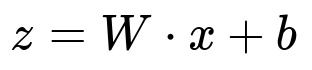
Here, W represents the learned weights associated with the connections leading into a hidden neuron, x is the input vector (which could be the original features or outputs from a previous hidden layer), and b is the bias term that shifts the activation. The next step is to apply a nonlinear activation function f, giving:

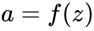
Where a is the output of that particular hidden neuron. By stacking multiple neurons, we form a hidden layer output vector, which then serves as the input to the subsequent layer. The nonlinear activation functions (such as ReLU, sigmoid, or tanh) play a critical role in allowing the network to approximate a wide variety of functions. Without these nonlinearities, the network would be limited to learning only linear transformations.

Within each hidden layer, the model captures increasingly high-level or abstract features. For example, if the input is an image, early hidden layers might detect simple edges or corners, while deeper hidden layers capture complex textures or shapes. This hierarchical representation is what makes deep neural networks capable of solving challenging tasks in computer vision, natural language processing, and other domains.

Why Multiple Hidden Layers Help

Multiple hidden layers, each equipped with its own set of weights and biases, deepen this representation-learning hierarchy. When you have many layers, the network can learn more nuanced patterns and handle highly complex relationships. However, adding more layers also introduces challenges like vanishing or exploding gradients, which can make training difficult. Techniques such as careful weight initialization, normalization layers (e.g., Batch Normalization), and skip connections (e.g., in ResNet architectures) help address these issues.

Practical Implementation Detail

In deep learning frameworks such as PyTorch or TensorFlow, you typically define each hidden layer as a linear (fully connected) transform followed by an activation. For instance, in PyTorch:

import torch
import torch.nn as nn

class SimpleNN(nn.Module):
    def __init__(self, input_dim, hidden_dim, output_dim):
        super(SimpleNN, self).__init__()
        self.fc1 = nn.Linear(input_dim, hidden_dim)
        self.activation = nn.ReLU()
        self.fc2 = nn.Linear(hidden_dim, output_dim)

    def forward(self, x):
        x = self.fc1(x)
        x = self.activation(x)
        x = self.fc2(x)
        return x

# Usage:
model = SimpleNN(input_dim=784, hidden_dim=128, output_dim=10)

In this example, fc1 is the first hidden layer, where the linear computation z = W*x + b is performed, and a ReLU activation is subsequently applied. Then the second linear layer (fc2) connects to the output. This structure showcases how hidden layers are implemented in code and emphasizes how each hidden layer learns its own representation of the data.

Common Interview Follow-Up Questions

How do different activation functions affect hidden layer computations?

Different activation functions can drastically alter what a hidden layer computes. Functions like ReLU allow sparse activations (only certain neurons remain active for specific inputs), which can help mitigate vanishing gradient problems and speed up training. Other activations, such as sigmoid, can be effective for binary classification tasks but might saturate, leading to slower training for deep networks. The choice of activation depends on the specific problem domain, architecture depth, and optimization concerns.

What happens if there are no hidden layers?

If a network has no hidden layers, it reduces to a simple linear or logistic regression model. This severely limits its capacity to capture complex nonlinear relationships in the data. Although such a network can still learn to separate data linearly or perform basic regression, it lacks the representational power of deeper networks.

Why is nonlinearity essential in hidden layers?

Without nonlinearity, multiple layers of linear transformations would collapse into an equivalent single linear transform. By introducing nonlinear activation functions, each hidden layer can learn intricate patterns in the data. This allows deep neural networks to be universal approximators of continuous functions under suitable conditions.

What challenges arise as we add more hidden layers?

Deeper networks can suffer from vanishing or exploding gradients, making training unstable or slow. Various regularization strategies (such as dropout, weight decay, or data augmentation) become important to prevent overfitting. Additionally, advanced techniques like residual connections or normalizations help maintain stable gradients when the network grows very deep.

How do we choose the number of neurons in a hidden layer?

There is no strict rule for determining the optimal number of neurons. In practice, it depends on the complexity of your dataset, the size of the input, the level of detail required in learned representations, and computational constraints. Increasing the number of neurons can capture more complex patterns but may also increase the risk of overfitting. Techniques like cross-validation, grid search, or more sophisticated hyperparameter optimization methods help find a good balance.

When does adding more hidden layers not help?

Beyond a certain point, adding more layers may lead to diminishing returns or even degrade performance if the architecture becomes too large or too difficult to train. Insufficient training data, weak regularization, or inadequate optimization methods might make deeper networks overfit or fail to converge. It is also possible that a simpler model generalizes better for some tasks, especially when data or resources are limited.

What are common approaches to combat overfitting in deeper networks?

Regularization methods like dropout randomly “switch off” certain neurons in training, forcing other neurons to learn more robust representations. Weight decay (L2 regularization) penalizes large weights, promoting simpler models. Early stopping halts training when validation loss stops improving, which can prevent the model from fitting noise. Data augmentation is often used, especially in computer vision or audio tasks, to effectively increase the size and diversity of the training set.

What is the role of initialization for hidden layers?

Weight initialization plays a key role in ensuring gradients flow properly. Poor initialization can lead to exploding or vanishing gradients, slowing down or even halting effective training. Techniques such as Xavier/Glorot initialization or He initialization are often used in modern deep learning frameworks to keep the scale of the outputs consistent across layers.

How do hidden layers learn to extract high-level features?

Hidden layers learn from backpropagation signals that show them how to adjust their weights to reduce the error between the network’s outputs and the desired targets. Early layers typically learn lower-level features, and successive layers learn increasingly complex or abstract features based on the outputs of previous layers. This hierarchical feature extraction is a hallmark of deep learning’s success in tasks like image and speech recognition.

Why do deeper networks often require large datasets?

Deeper networks have more parameters, which allows them to represent highly complex functions. However, each parameter must be learned from data. If there is not enough training data, the model can memorize noise instead of learning generalizable patterns, leading to overfitting. Larger datasets help networks learn robust, generalizable representations at multiple levels of abstraction.

Does the shape of the hidden layers matter more than depth?

The shape of each hidden layer (its width) and the number of layers (its depth) both matter. A network might be deep (many layers) but with relatively small layers, or shallow (fewer layers) but with many neurons per layer. In practice, the optimal shape depends on the task and data. Some architectures favor deeper but narrower layers, while others benefit from shallower but wider layers.

These considerations illustrate why the computations in a hidden layer are the foundation of a neural network’s power. By combining linear transformations with nonlinear activations, hidden layers enable deep networks to learn high-level abstractions needed for a wide range of complex tasks.

Below are additional follow-up questions

How do hidden layers handle data with many missing values or noise?

Hidden layers are not inherently designed to fix missing data or denoise signals on their own; they learn whatever patterns the training process allows them to extract. If there are many missing values, the network may pick up spurious correlations or fail to converge if preprocessing steps are not done carefully. When data is noisy, the model might overfit those noise patterns, especially if there are insufficient regularization strategies in place. In real-world scenarios, it is common to handle missing values through imputation (for instance, mean or median imputation, or more advanced approaches like k-nearest neighbors) before feeding data into the network. Denoising can also be approached through specialized architectures such as denoising autoencoders, which explicitly learn to reconstruct clean representations from noisy inputs. Another pitfall arises when different columns in tabular data have significantly varying levels of missingness, leading certain neurons to get “overloaded” by unreliable features. Careful feature engineering, thorough data cleaning, and domain-specific transformations can mitigate these issues.

What is the difference between feed-forward hidden layers and recurrent hidden layers in terms of computations and potential pitfalls?

Feed-forward hidden layers process data in a single pass, treating each input independently. This is well-suited for tasks like static image classification or tabular data regression. Recurrent hidden layers, in contrast, process sequential or temporal data by retaining hidden states that carry information from previous time steps. This allows them to capture context over time, making them essential for tasks such as language modeling or time-series forecasting. However, recurrent architectures can be more difficult to train due to issues like vanishing and exploding gradients over longer sequences. Techniques like gating mechanisms (LSTM or GRU), gradient clipping, and proper initialization help mitigate these pitfalls. Another subtlety is that feed-forward networks usually train faster and scale more easily on parallel hardware like GPUs, while recurrent layers often require specialized operations that can be more complex to optimize efficiently at scale.

How do skip connections, as used in ResNet or DenseNet, affect hidden layer computations?

Skip connections allow activations from earlier layers to “skip” forward to deeper layers. This helps mitigate vanishing gradients, because gradients have a direct pathway back to earlier layers. In a ResNet block, the output of a hidden layer is added to the output of a deeper layer, effectively creating a shortcut for both forward pass information and backward pass gradients. This modification often leads to better optimization properties and improved training convergence in very deep architectures. A subtle side effect is that some neurons in deeper layers can bypass transformations if the shortcut path dominates, but in practice this usually provides a helpful ensemble-like effect, allowing the model to learn both shallow and deep representations. In DenseNet architectures, skip connections feed the feature maps from all preceding layers to each subsequent layer, further enriching the representation in a computationally efficient way.

How do we interpret or visualize what hidden layers have learned?

Interpreting hidden layers can be challenging, especially in high-dimensional and high-depth networks. Techniques like activation maximization aim to synthesize an input that strongly activates certain neurons, revealing what those neurons respond to. Another approach is to use dimensionality reduction (e.g., t-SNE or PCA) on the activation outputs of a hidden layer to see if the network clusters similar inputs together. For image-based tasks, saliency maps or more advanced methods like Grad-CAM can help visualize which regions of the input image influence specific activations. In NLP, techniques may involve analyzing attention weights (in Transformer-based models) or hidden state trajectories (in LSTM-based models). A common pitfall arises when we assume these interpretations fully explain the model’s decision-making; in reality, they only provide approximate insights and can be misled by complex interactions across many neurons.

Are there scenarios where smaller or narrower hidden layers outperform deeper or wider ones?

Sometimes, a simpler network with fewer neurons per layer can outperform a deeper or wider counterpart due to better generalization when the dataset is small or when the underlying function is not overly complex. Overly large networks may memorize the training data’s noise instead of capturing generalizable patterns. Another subtle scenario is when computational constraints or latency requirements dictate that a smaller model is preferable, even if a larger one might achieve slightly better accuracy. In industrial applications like mobile or real-time inference, a compact network is often chosen to meet strict performance requirements. Pruning and quantization can also reduce model size while retaining most of the performance benefits of deeper networks.

How do hidden layers in a neural network behave differently when used in a reinforcement learning context?

In reinforcement learning (RL), the hidden layers learn policies or value functions that depend on sequential decision-making rather than straightforward classification or regression. The network’s parameters are updated based on reward signals that might be sparse or delayed. Because of this, hidden layers in RL might need to capture both short-term cues (e.g., immediate sensor inputs in a game) and long-term strategies (e.g., states that indicate future reward potential). Challenges arise if the reward is too delayed, which can lead to unstable training or insufficient gradient signals to update hidden layer weights effectively. Algorithms such as Deep Q-Network (DQN) handle this by using replay buffers and target networks, helping reduce correlations in consecutive state transitions and stabilizing the training process. Nonetheless, hidden layer representations in RL can oscillate or fail to converge if hyperparameters or exploration strategies are poorly chosen.

What role does layer normalization or batch normalization play in stabilizing hidden layer outputs?

Normalization techniques like batch normalization or layer normalization address the internal covariate shift problem, where the distribution of activations in hidden layers changes during training, making it difficult to converge. By normalizing activations, the network reduces sensitivity to weight initialization and allows for higher learning rates. Batch normalization does this across each mini-batch dimension, while layer normalization normalizes each feature dimension for a single sample. In practice, this helps stabilize training, speed up convergence, and often improves generalization. Potential pitfalls include small batch sizes, where batch statistics might become unreliable, or mismatch between training and inference distributions if the network relies too heavily on batch statistics. Also, for recurrent networks, batch normalization can sometimes introduce dependencies between time steps, so layer normalization is often preferred for RNNs.

How do transformer-based architectures structure their hidden layers differently from traditional feed-forward networks?

Transformers use a stack of self-attention and feed-forward sub-layers, each wrapped in layer normalization and equipped with residual connections. In these architectures, the hidden layers learn to capture relationships among all positions in a sequence through attention mechanisms rather than relying solely on fixed receptive fields (as in CNNs) or sequential hidden state updates (as in RNNs). This approach allows for parallel processing of the entire input sequence, which can significantly speed up training on large datasets. A unique pitfall is the quadratic computational complexity in the sequence length, limiting the size of inputs that can be processed efficiently. Furthermore, the multi-head self-attention mechanism may inadvertently focus on unimportant parts of the sequence if not well-trained or if regularization methods (like dropout) are insufficient.

Why might a hidden layer become “idle” or “dead” during training, and what can be done about it?

A neuron can become “dead” if its weights and bias cause it to output zero (for ReLU) or a saturated region (for sigmoid or tanh) for most inputs, and subsequently, it receives near-zero gradients. In such a state, the neuron stops updating effectively and contributes little to the learned representation. This issue is relatively common with ReLU activations, where negative inputs result in zero outputs and zero gradients. Solutions include careful initialization to reduce the chance of all inputs being negative, using activation variants like Leaky ReLU or ELU that allow a small gradient to flow when inputs are negative, and employing normalization layers so that distributions of neuron inputs remain in a more active region. If a large fraction of neurons become dead, it can severely limit the model’s capacity, so monitoring the activation statistics during training can help catch this problem early.

Can hidden layers cause an internal covariate shift, and how does it affect training?

Yes, internal covariate shift refers to the change in the distribution of inputs to each hidden layer as the parameters of the previous layers change during training. This shift makes training deeper networks harder, as the next layer must constantly adapt to a moving target distribution. Batch normalization and other normalization techniques were introduced partly to reduce internal covariate shift by normalizing layer inputs, helping the network train faster and more stably. However, if batch sizes are too small or if data is not well-shuffled, the computed normalization statistics can be noisy, causing training instability. Additionally, as the model becomes very deep, even small changes in layer distributions can accumulate and lead to convergence difficulties. Monitoring training metrics and conducting careful hyperparameter tuning are key to mitigating this issue.